MATLAB Tutorial
Welcome to the MATLAB tutorial version of Data Science Rosetta Stone. Before beginning this tutorial, please check to make sure you have MATLAB installed.
Note: In MATLAB,
% This is a single line comment.
%{ This is a paragraph
comment %}
Now let’s get started!
1 Reading in Data and Basic Statistical Functions
1.1 Read in the data.
a) Read the data in as a .csv file.
First specify the format of the variables to be read in: %C = character, %d = integer, %f = floating point number.
formatSpec = '%C%C%d%f%f';
student = readtable('class.csv', 'Delimiter', ',', 'Format', formatSpec);
b) Read the data in as a .xls file.
MATLAB reads tables from .xlsx formats, which is another version of an Excel file.
student_xlsx = readtable('class.xlsx');
c) Read the data in as a .json file.
student_json = jsondecode(fileread('class.json'));
1.2 Find the dimensions of the data set.
1.3 Find basic information about the data set.
summary(student);
Variables:

    Name: 19×1 categorical

        Values:

            Alfred     1
            Alice      1
            Barbara    1
            Carol      1
            Henry      1
            James      1
            Jane       1
            Janet      1
            Jeffrey    1
            John       1
            Joyce      1
            Judy       1
            Louise     1
            Mary       1
            Philip     1
            Robert     1
            Ronald     1
            Thomas     1
            William    1

    Sex: 19×1 categorical

        Values:

            F     9
            M    10

    Age: 19×1 int32

        Values:

            Min       11
            Median    13
            Max       16

    Height: 19×1 double

        Values:

            Min       51.3
            Median    62.8
            Max         72

    Weight: 19×1 double

        Values:

            Min       50.5
            Median    99.5
            Max        150
summary()
1.4 Look at the first 5 (last 5) observations.
The ":" operator tells MATLAB to print all columns (variables), while "1:5" indicates to print only the first 5 observations.
disp(student(1:5,:));
     Name      Sex    Age    Height    Weight
    _______    ___    ___    ______    ______

    Alfred     M      14       69      112.5
    Alice      F      13     56.5         84
    Barbara    F      13     65.3         98
    Carol      F      14     62.8      102.5
    Henry      M      14     63.5      102.5
disp()
1.5 Calculate means of numeric variables.
age = table2array(student(:,3));
disp(mean(age));
13.3158
height = table2array(student(:,4));
disp(mean(height));
62.3368
weight = table2array(student(:,5));
disp(mean(weight));
100.0263table2array() | mean() | disp()
1.6 Compute summary statistics of the data set.
numeric_vars = student(:,{'Age', 'Height', 'Weight'});
statarray = grpstats(numeric_vars, [], {'min', 'median', 'mean', 'max'});
disp(statarray);
           GroupCount    min_Age    median_Age    mean_Age    max_Age    min_Height    median_Height    mean_Height    max_Height    min_Weight    median_Weight    mean_Weight    max_Weight
           __________    _______    __________    ________    _______    __________    _____________    ___________    __________    __________    _____________    ___________    __________

    All    19            11         13            13.316      16         51.3          62.8             62.337         72            50.5          99.5             100.03         150
grpstats() | disp()
1.7 Descriptive statistics functions applied to variables of the data set.
weight = table2array(student(:,5));
disp(std(weight));
22.7739
disp(sum(weight));
1.9005e+03
disp(length(weight));
19
disp(max(weight));
150
disp(min(weight));
50.5000
disp(median(weight));
99.5000table2array() | std() | sum() | length() | max() | min() | median()
1.8 Produce a one-way table to describe the frequency of a variable.
a) Produce a one-way table of a discrete variable.
tabulate(age);
  Value    Count   Percent
      1        0      0.00%
      2        0      0.00%
      3        0      0.00%
      4        0      0.00%
      5        0      0.00%
      6        0      0.00%
      7        0      0.00%
      8        0      0.00%
      9        0      0.00%
     10        0      0.00%
     11        2     10.53%
     12        5     26.32%
     13        3     15.79%
     14        4     21.05%
     15        4     21.05%
     16        1      5.26%
tabulate()
b) Produce a one-way table of a categorical variable.
sex = table2array(student(:,{'Sex'}));
tabulate(sex);
  Value    Count   Percent
      F        9     47.37%
      M       10     52.63%
1.9 Produce a two-way table to describe the frequency of two categorical or discrete variables.
crosstable = varfun(@(x) length(x), student, 'GroupingVariables', {'Age' 'Sex'}, 'InputVariables', {});
disp(crosstable);
    Age    Sex    GroupCount
    ___    ___    __________

    11     F      1
    11     M      1
    12     F      2
    12     M      3
    13     F      2
    13     M      1
    14     F      2
    14     M      2
    15     F      2
    15     M      2
    16     M      1
varfun()
1.10 Select a subset of the data that meets a certain criterion.
% Find the indices of those students who are females, and then get those observations
% from the student data frame.
females = student(student.Sex == 'F',:);
disp(females(1:5,:));
     Name      Sex    Age    Height    Weight
    _______    ___    ___    ______    ______

    Alice      F      13     56.5         84
    Barbara    F      13     65.3         98
    Carol      F      14     62.8      102.5
    Jane       F      12     59.8       84.5
    Janet      F      15     62.5      112.5
1.11 Determine the correlation between two continuous variables.
The first argument of the cat function is dim, which is specified as 2 here to indicate to concatenate column-wise.
height_weight = cat(2,table2array(student(:,4)),table2array(student(:,5)));
disp(corr(height_weight));
    1.0000    0.8778
    0.8778    1.0000
table2array() | cat() | corr()
2 Basic Graphing and Plotting Functions
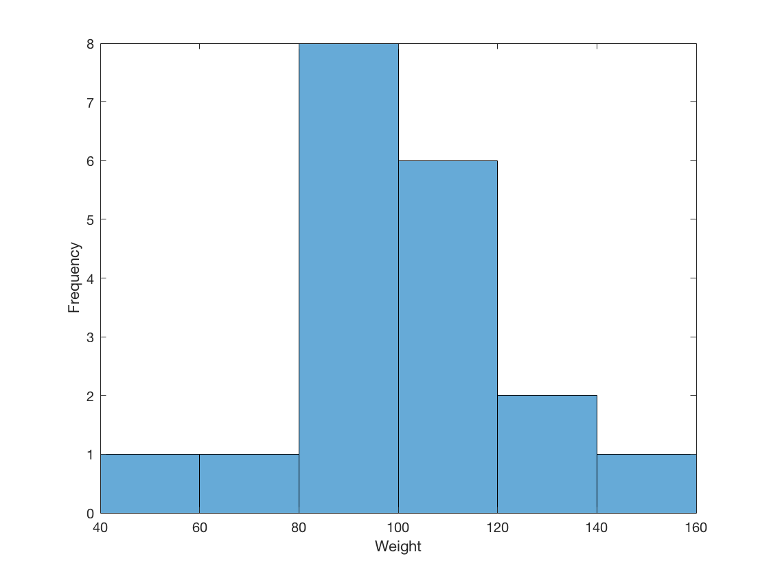
2.1 Visualize a single continuous variable by producing a histogram.
Weight = table2array(student(:,{'Weight'}));
histogram(Weight, 40:20:160)
xlabel('Weight');
ylabel('Frequency');
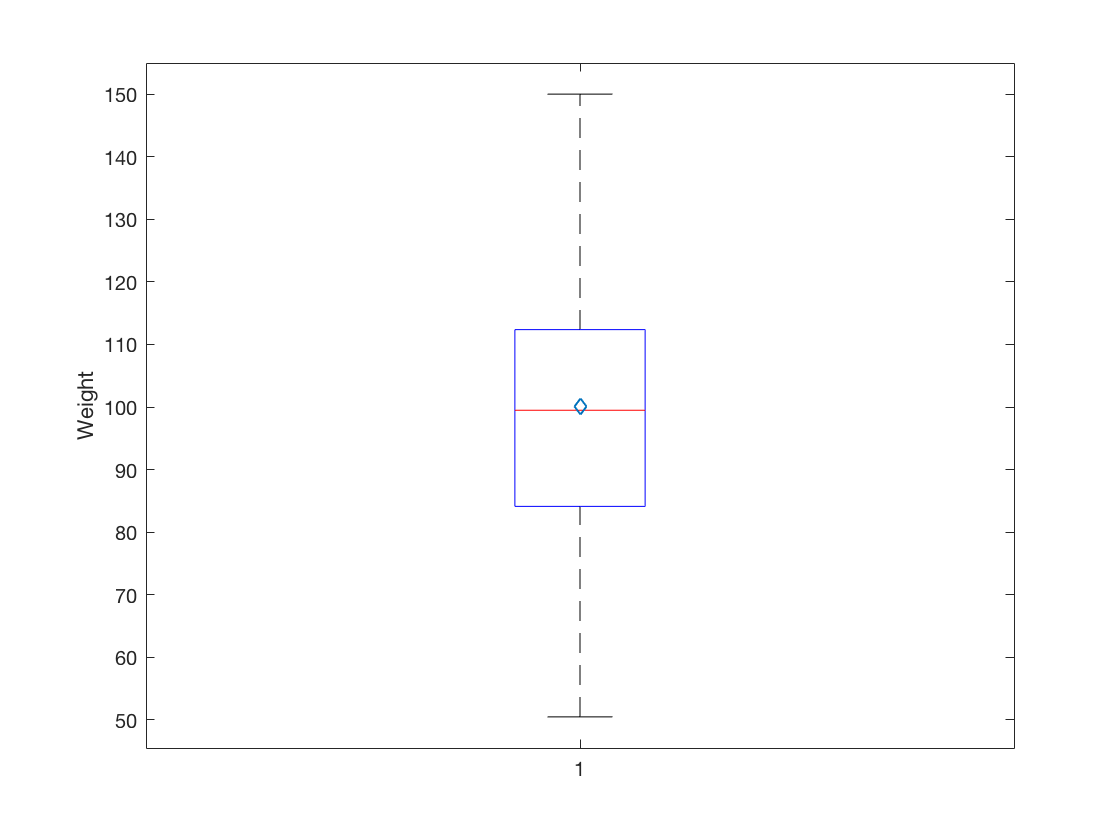
2.2 Visualize a single continuous variable by producing a boxplot.
boxplot(Weight);
mx = mean(Weight);
ylabel('Weight');
hold on
plot(mx, 'd')
hold off
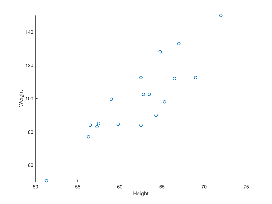
2.3 Visualize two continuous variables by producing a scatterplot.
Height = table2array(student(:,{'Height'}));
scatter(Height, Weight)
xticks(50:5:75)
yticks(40:20:160)
xlabel('Height')
ylabel('Weight')
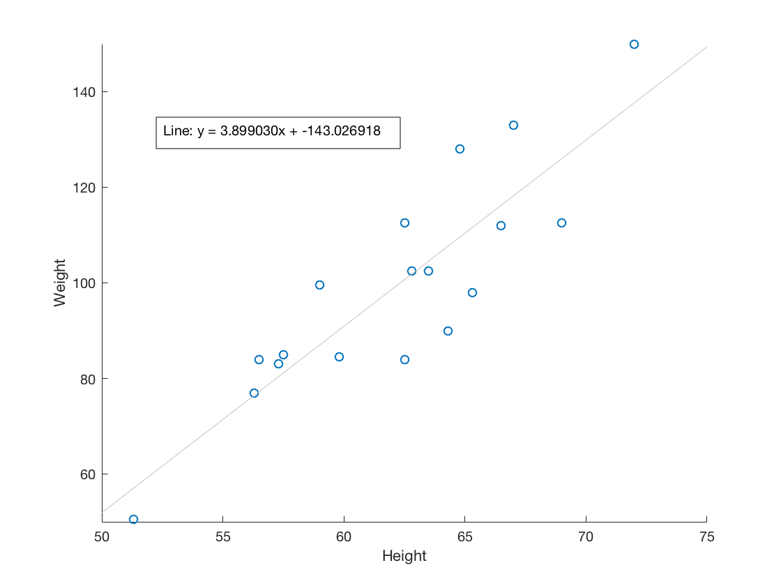
2.4 Visualize a relationship between two continuous variables by producing a scatterplot and a plotted line of best fit.
scatter(Height, Weight)
xticks(50:5:75)
yticks(40:20:160)
xlabel('Height')
ylabel('Weight')
b = polyfit(Height, Weight,1);
m = b(1);
y_int = b(2);
lsline
annotation('textbox', [.2 .5 .3 .3], 'String', sprintf('Line: y = %fx + %f', m, y_int), ...
    'FitBoxToText', 'on');
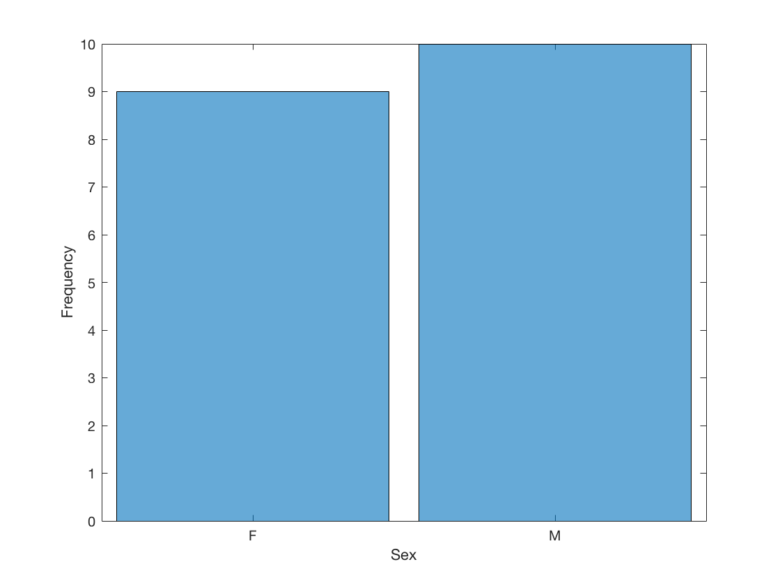
2.5 Visualize a categorical variable by producing a bar chart.
Sex = table2array(student(:,{'Sex'}));
histogram(Sex)
xlabel('Sex')
ylabel('Frequency')
2.6 Visualize a continuous variable, grouped by a categorical variable, by producing side-by-side boxplots.
females = student(student.Sex == 'F',:);
males = student(student.Sex == 'M',:);
Female_Weight = table2array(females(:,{'Weight'}));
Male_Weight = table2array(males(:,{'Weight'}));
clf
boxplot(Weight, Sex);
means = [mean(Female_Weight), mean(Male_Weight)];
xlabel('Sex');
ylabel('Weight');
hold on
plot(means, 'd')
hold off

3 Basic Data Wrangling and Manipulation
3.1 Create a new variable in a data set as a function of existing variables in the data set.
% The "./" (and similarly, ".^2") tells MATLAB to divide (and similarly, exponentiate)
% element-wise, instead of matrix-wise.
student.BMI = student.Weight ./ student.Height .^ 2 * 703;
disp(student(1:5,:));
     Name      Sex    Age    Height    Weight     BMI
    _______    ___    ___    ______    ______    ______

    Alfred     M      14       69      112.5     16.612
    Alice      F      13     56.5         84     18.499
    Barbara    F      13     65.3         98     16.157
    Carol      F      14     62.8      102.5     18.271
    Henry      M      14     63.5      102.5      17.87
3.2 Create a new variable in a data set using if/else logic of existing variables in the data set.
student.BMI_Class = student.Name;
for i = 1:size(student,1)
    if student.BMI(i) < 19.0
        student.BMI_Class(i) = 'Underweight';
    else
        student.BMI_Class(i) = 'Healthy';
    end
end
disp(student(1:5,:));
     Name      Sex    Age    Height    Weight     BMI       BMI_Class
    _______    ___    ___    ______    ______    ______    ___________

    Alfred     M      14       69      112.5     16.612    Underweight
    Alice      F      13     56.5         84     18.499    Underweight
    Barbara    F      13     65.3         98     16.157    Underweight
    Carol      F      14     62.8      102.5     18.271    Underweight
    Henry      M      14     63.5      102.5      17.87    Underweight
3.3 Create new variables in a data set using mathematical functions applied to existing variables in the data set.
student.LogWeight = log(student.Weight);
student.ExpAge = exp(double(student.Age));
student.SqrtHeight = sqrt(student.Height);
student.BMI_Neg = student.BMI;
for i = 1:size(student,1)
    if student.BMI(i) < 19.0
        student.BMI_Neg(i) = -student.BMI(i);
    end
end
student.BMI_Pos = abs(student.BMI_Neg);
student.BMI_Check = (student.BMI_Pos == student.BMI);
disp(student(1:5,:));
     Name      Sex    Age    Height    Weight     BMI       BMI_Class     LogWeight      ExpAge      SqrtHeight    BMI_Neg    BMI_Pos    BMI_Check
    _______    ___    ___    ______    ______    ______    ___________    _________    __________    __________    _______    _______    _________

    Alfred     M      14       69      112.5     16.612    Underweight     4.723       1.2026e+06    8.3066        -16.612    16.612     true
    Alice      F      13     56.5         84     18.499    Underweight    4.4308       4.4241e+05    7.5166        -18.499    18.499     true
    Barbara    F      13     65.3         98     16.157    Underweight     4.585       4.4241e+05    8.0808        -16.157    16.157     true
    Carol      F      14     62.8      102.5     18.271    Underweight    4.6299       1.2026e+06    7.9246        -18.271    18.271     true
    Henry      M      14     63.5      102.5      17.87    Underweight    4.6299       1.2026e+06    7.9687         -17.87     17.87     true
log() | exp() | sqrt() | abs()
3.4 Drop variables from a data set.
Setting the variables to an empty array deletes the variables from the dataset.
student.LogWeight = [];
student.ExpAge = [];
student.SqrtHeight = [];
student.BMI_Neg = [];
student.BMI_Pos = [];
student.BMI_Check = [];
disp(student(1:5,:));
     Name      Sex    Age    Height    Weight     BMI       BMI_Class
    _______    ___    ___    ______    ______    ______    ___________

    Alfred     M      14       69      112.5     16.612    Underweight
    Alice      F      13     56.5         84     18.499    Underweight
    Barbara    F      13     65.3         98     16.157    Underweight
    Carol      F      14     62.8      102.5     18.271    Underweight
    Henry      M      14     63.5      102.5      17.87    Underweight
3.5 Sort a data set by a variable.
a) Sort data set by a continuous variable.
student = sortrows(student, 'Age');
disp(student(1:5,:));
    Name     Sex    Age    Height    Weight     BMI       BMI_Class
    ______    ___    ___    ______    ______    ______    ___________

    Joyce     F      11     51.3      50.5       13.49    Underweight
    Thomas    M      11     57.5        85      18.073    Underweight
    James     M      12     57.3        83      17.772    Underweight
    Jane      F      12     59.8      84.5      16.612    Underweight
    John      M      12       59      99.5      20.094    Healthy
sortrows()
b) Sort data set by a categorical variable.
student = sortrows(student, 'Sex');
disp(student(1:5,:));
    Name      Sex    Age    Height    Weight     BMI       BMI_Class
    _______    ___    ___    ______    ______    ______    ___________

    Joyce      F      11     51.3      50.5       13.49    Underweight
    Jane       F      12     59.8      84.5      16.612    Underweight
    Louise     F      12     56.3        77      17.078    Underweight
    Alice      F      13     56.5        84      18.499    Underweight
    Barbara    F      13     65.3        98      16.157    Underweight
sortrows()
3.6 Compute descriptive statistics of continuous variables, grouped by a categorical variable.
group_means = grpstats(student, 'Sex', 'mean', 'DataVars', {'Age', 'Height', 'Weight', 'BMI'});
disp(group_means);
         Sex    GroupCount    mean_Age    mean_Height    mean_Weight    mean_BMI
         ___    __________    ________    ___________    ___________    ________

    F    F       9            13.222      60.589         90.111         17.051
    M    M      10              13.4       63.91         108.95         18.594
grpstats()
3.7 Add a new row to the bottom of a data set.
disp(student(15:19,:));
     Name      Sex    Age    Height    Weight     BMI       BMI_Class
    _______    ___    ___    ______    ______    ______    ___________

    Alfred     M      14       69      112.5     16.612    Underweight
    Henry      M      14     63.5      102.5      17.87    Underweight
    Ronald     M      15       67        133     20.828    Healthy
    William    M      15     66.5        112     17.805    Underweight
    Philip     M      16       72        150     20.341    Healthy
newObs = {'Name', 'Sex', 'Age', 'Height', 'Weight', 'BMI', 'BMI_Class';
    'Jane', 'F', 14, 56.3, 77.0, 17.077695, 'Underweight'};
newTable = dataset2table(cell2dataset(newObs));
student = vertcat(student,newTable);
disp(student(16:20,:));
     Name      Sex    Age    Height    Weight     BMI       BMI_Class
    _______    ___    ___    ______    ______    ______    ___________

    Henry      M      14     63.5      102.5      17.87    Underweight
    Ronald     M      15       67        133     20.828    Healthy
    William    M      15     66.5        112     17.805    Underweight
    Philip     M      16       72        150     20.341    Healthy
    Jane       F      14     56.3         77     17.078    Underweight
cell2dataset() | dataset2table() | vertcat()
3.8 Create a user-defined function and apply it to a variable in the data set to create a new variable in the data set.
% To create a user-defined function, create a new file in MATLAB with the function definition,
% and save the file as the function_name.m.  Here, toKG.m would be:
%
% function KG = toKG(lb);
%          KG = 0.45359237 * lb;
% end
student.Weight_KG = toKG(student.Weight);
disp(student(1:5,:));
     Name      Sex    Age    Height    Weight     BMI       BMI_Class     Weight_KG
    _______    ___    ___    ______    ______    ______    ___________    _________

    Joyce      F      11     51.3      50.5       13.49    Underweight    22.906
    Jane       F      12     59.8      84.5      16.612    Underweight    38.329
    Louise     F      12     56.3        77      17.078    Underweight    34.927
    Alice      F      13     56.5        84      18.499    Underweight    38.102
    Barbara    F      13     65.3        98      16.157    Underweight    44.452
user-defined function
4 More Advanced Data Wrangling
4.1 Drop observations with missing information.
formatSpec = '%C%f%f%f%f%f%f';
fish = readtable('fish.csv', 'Delimiter', ',', ...
    'Format', formatSpec);
fish = sortrows(fish, 'Weight', 'descend');
disp(fish(1:5,:));
    Species    Weight    Length1    Length2    Length3    Height    Width
    _______    ______    _______    _______    _______    ______    ______

    Bream       NaN      29.5         32       37.3       13.913    5.0728
    Pike       1650        59       63.4         68       10.812      7.48
    Pike       1600        56         60         64          9.6     6.144
    Pike       1550        56         60         64          9.6     6.144
    Pike       1250        52         56       59.7       10.686    6.9849
fish = rmmissing(fish);
disp(fish(1:5,:));
    Species    Weight    Length1    Length2    Length3    Height    Width
    _______    ______    _______    _______    _______    ______    ______

    Pike       1650      59         63.4         68       10.812      7.48
    Pike       1600      56           60         64          9.6     6.144
    Pike       1550      56           60         64          9.6     6.144
    Pike       1250      52           56       59.7       10.686    6.9849
    Perch      1100      39           42       44.6         12.8    6.8684
readtable() | sortrows() | rmmissing()
4.2 Merge two data sets together on a common variable.
a) First, select specific columns of a data set to create two smaller data sets.
formatSpec = '%C%C%d%f%f';
student = readtable('class.csv', 'Delimiter', ',', ...
    'Format', formatSpec);
student1 = student(:, {'Name', 'Sex', 'Age'});
disp(student1(1:5,:));
     Name      Sex    Age
    _______    ___    ___

    Alfred     M      14
    Alice      F      13
    Barbara    F      13
    Carol      F      14
    Henry      M      14
student2 = student(:, {'Name', 'Height', 'Weight'});
disp(student2(1:5,:));
     Name      Height    Weight
    _______    ______    ______

    Alfred       69      112.5
    Alice      56.5         84
    Barbara    65.3         98
    Carol      62.8      102.5
    Henry      63.5      102.5
readtable()
b) Second, we want to merge the two smaller data sets on the common variable.
new = join(student1, student2);
disp(new(1:5,:));
     Name      Sex    Age    Height    Weight
    _______    ___    ___    ______    ______

    Alfred     M      14       69      112.5
    Alice      F      13     56.5         84
    Barbara    F      13     65.3         98
    Carol      F      14     62.8      102.5
    Henry      M      14     63.5      102.5
join()
c) Finally, we want to check to see if the merged data set is the same as the original data set.
4.3 Merge two data sets together by index number only.
a) First, select specific columns of a data set to create two smaller data sets.
newstudent1 = student(:, {'Name', 'Sex', 'Age'});
disp(newstudent1(1:5,:));
     Name      Sex    Age
    _______    ___    ___

    Alfred     M      14
    Alice      F      13
    Barbara    F      13
    Carol      F      14
    Henry      M      14
newstudent2 = student(:, {'Height', 'Weight'});
disp(newstudent2(1:5,:));
    Height    Weight
    ______    ______

      69      112.5
    56.5         84
    65.3         98
    62.8      102.5
    63.5      102.5
b) Second, we want to join the two smaller data sets.
new2 = [newstudent1, newstudent2];
disp(new2(1:5,:));
     Name      Sex    Age    Height    Weight
    _______    ___    ___    ______    ______

    Alfred     M      14       69      112.5
    Alice      F      13     56.5         84
    Barbara    F      13     65.3         98
    Carol      F      14     62.8      102.5
    Henry      M      14     63.5      102.5
c) Finally, we want to check to see if the joined data set is the same as the original data set.
4.4 Create a pivot table to summarize information about a data set.
% Currently there is not a MATLAB function for creating pivot tables, but only user-defined functions
% that could be used to create pivot tables.
pivottable user-defined function
4.5 Return all unique values from a text variable.
price = readtable('price.xlsx');
disp(unique(price.STATE));
    'Baja California Norte'
    'British Columbia'
    'California'
    'Campeche'
    'Colorado'
    'Florida'
    'Illinois'
    'Michoacan'
    'New York'
    'North Carolina'
    'Nuevo Leon'
    'Ontario'
    'Quebec'
    'Saskatchewan'
    'Texas'
    'Washington'
readtable() | unique()5 Preparation & Basic Regression
5.1 Pre-process a data set using principal component analysis.
formatSpec = '%f%f%f%f%d';
iris = readtable('iris.csv', 'Delimiter', ',', ...
    'Format', formatSpec);
features = table2array(iris(:, {'SepalLength', 'SepalWidth', 'PetalLength', 'PetalWidth'}));
% Z-score function to scale
Zsc = @(x) (x-mean(x))./std(x);
features_scaled = Zsc(features);
disp(pca(features_scaled));
    0.5224    0.3723    0.7210   -0.2620
   -0.2634    0.9256   -0.2420    0.1241
    0.5813    0.0211   -0.1409    0.8012
    0.5656    0.0654   -0.6338   -0.5235
readtable() | table2array() | pca()
5.2 Split data into training and testing data and export as a .csv file.
sizeIris = size(iris);
numRows = sizeIris(1);
% Set the seed of the random number generator
% for reproducibility.
rng(29);
[trainInd, valInd, testInd] = dividerand(numRows, 0.7, 0, 0.3);
train = iris(trainInd,:);
test = iris(testInd,:);
csvwrite('iris_train_ML.csv', table2array(train));
csvwrite('iris_test_ML.csv', table2array(test));
size() | rng() | dividerand() | table2array() | csvwrite()
5.3 Fit a logistic regression model.
formatSpec = '%d%f%f%C%C%C%C%d';
tips = readtable('tips.csv', 'Delimiter', ',', ...
    'Format', formatSpec);
tips.fifteen = 0.15 * tips.total_bill;
tips.greater15 = (tips.tip > tips.fifteen);
[b, dev, stats] = glmfit(tips.total_bill, tips.greater15, 'binomial', 'link', 'logit');
fprintf('The coefficients of the model are: %.3f and %.3f\n', b(1), b(2));
fprintf('The deviance of the fit of the fit is: %.3f\n', dev);
fprintf('Other statistics of the model are:\n');
disp(stats);
The coefficients of the model are: 1.648 and -0.072
The deviance of the fit of the fit is: 313.743
Other statistics of the model are:
         beta: [2×1 double]
          dfe: 242
         sfit: 1.0097
            s: 1
      estdisp: 0
         covb: [2×2 double]
           se: [2×1 double]
    coeffcorr: [2×2 double]
            t: [2×1 double]
            p: [2×1 double]
        resid: [244×1 double]
       residp: [244×1 double]
       residd: [244×1 double]
       resida: [244×1 double]
          wts: [244×1 double]
readtable() | glmfit() | fprintf()
5.4 Fit a linear regression model.
linreg = fitlm(tips,'tip~total_bill');
disp(linreg);
Linear regression model:
    tip ~ 1 + total_bill

Estimated Coefficients:
                   Estimate       SE        tStat       pValue
                   ________    _________    ______    __________

    (Intercept)    0.92027       0.15973    5.7612    2.5264e-08
    total_bill     0.10502     0.0073648     14.26    6.6925e-34


Number of observations: 244, Error degrees of freedom: 242
Root Mean Squared Error: 1.02
R-squared: 0.457,  Adjusted R-Squared 0.454
F-statistic vs. constant model: 203, p-value = 6.69e-34
fitlm()
6 Supervised Machine Learning
6.1 Fit a logistic regression model on training data and assess against testing data.
a) Fit a logistic regression model on training data.
formatSpec = '%f%d%d%d%f';
train = readtable('tips_train.csv', 'Delimiter', ',', ...
    'Format', formatSpec);
test = readtable('tips_test.csv', 'Delimiter', ',', ...
    'Format', formatSpec);
train.fifteen = 0.15 * train.total_bill;
train.greater15 = (train.tip > train.fifteen);
test.fifteen = 0.15 * test.total_bill;
test.greater15 = (test.tip > test.fifteen);
[b, dev, stats] = glmfit(train.total_bill, train.greater15, 'binomial', 'link', 'logit');
fprintf('The coefficients of the model are: %.3f and %.3f\n', b(1), b(2));
fprintf('The deviance of the fit of the fit is: %.3f\n', dev);
fprintf('Other statistics of the model are:\n');
disp(stats);
The coefficients of the model are: 1.646 and -0.071
The deviance of the fit of the fit is: 250.584
Other statistics of the model are:
         beta: [2×1 double]
          dfe: 193
         sfit: 1.0107
            s: 1
      estdisp: 0
         covb: [2×2 double]
           se: [2×1 double]
    coeffcorr: [2×2 double]
            t: [2×1 double]
            p: [2×1 double]
        resid: [195×1 double]
       residp: [195×1 double]
       residd: [195×1 double]
       resida: [195×1 double]
          wts: [195×1 double]
readtable() | glmfit() | fprintf()
b) Assess the model against the testing data.
predictions = glmval(b, test.total_bill, 'logit');
predY = round(predictions);
Results = strings(size(test,1),1);
for i = 1:size(test,1)
    if (predY(i) == test.greater15(i))
        Results(i) = 'Correct';
    else
        Results(i) = 'Wrong';
    end
end
tabulate(Results);
    Value    Count   Percent
  Correct       34     69.39%
    Wrong       15     30.61%
glmval() | round() | size() | strings() | tabulate()
6.2 Fit a linear regression model on training data and assess against testing data.
a) Fit a linear regression model on training data.
train = readtable('boston_train.xlsx');
test = readtable('boston_test.xlsx');
x_train = train;
x_train.Target = [];
y_train = train.Target;
x_test = test;
x_test.Target = [];
y_test = test.Target;
linreg = fitlm(table2array(x_train), y_train);
disp(linreg);
Linear regression model:
    y ~ 1 + x1 + x2 + x3 + x4 + x5 + x6 + x7 + x8 + x9 + x10 + x11 + x12 + x13

Estimated Coefficients:
                    Estimate        SE         tStat        pValue
                   __________    _________    ________    __________

    (Intercept)        36.108        6.505      5.5509    5.7321e-08
    x1              -0.085634     0.042774      -2.002      0.046077
    x2               0.046034      0.01715      2.6842     0.0076262
    x3               0.036413     0.076006     0.47909       0.63219
    x4                  3.248       1.0741      3.0238     0.0026862
    x5                -14.873       4.6361     -3.2081     0.0014633
    x6                 3.5769      0.53699      6.6609    1.0962e-10
    x7             -0.0087032     0.016853    -0.51643       0.60589
    x8                -1.3689      0.25296     -5.4115    1.1818e-07
    x9                0.31312     0.082366      3.8016    0.00017037
    x10             -0.012882    0.0045986     -2.8012     0.0053829
    x11               -0.9769        0.171      -5.713    2.4255e-08
    x12              0.011326    0.0033585      3.3722    0.00083155
    x13              -0.52672     0.062563      -8.419    1.0751e-15

Number of observations: 354, Error degrees of freedom: 340
Root Mean Squared Error: 4.99
R-squared: 0.724,  Adjusted R-Squared 0.713
F-statistic vs. constant model: 68.5, p-value = 1.39e-86
readtable() | fitlm()
b) Assess the model against the testing data.
predictions = predict(linreg, table2array(x_test));
sq_diff = (predictions - y_test) .^ 2;
disp(mean(sq_diff));
17.7713
6.3 Fit a decision tree model on training data and assess against testing data.
a) Fit a decision tree classification model.
i) Fit a decision tree classification model on training data and determine variable importance.
train = readtable('breastcancer_train.xlsx');
test = readtable('breastcancer_test.xlsx');
x_train = train;
x_train.Target = [];
y_train = train.Target;
x_test = test;
x_test.Target = [];
y_test = test.Target;
rng(29);
treeMod = fitctree(x_train, y_train);
var_import = predictorImportance(treeMod);
var_import = var_import';
var_import(:,2) = var_import;
for i = 1:size(var_import,1)
    var_import(i,1) = i;
end
var_import = sortrows(var_import, 2, 'descend');
disp(var_import(1:5,:));
   24.0000    0.0292
   28.0000    0.0077
    2.0000    0.0019
   12.0000    0.0013
    5.0000    0.0009
readtable() | rng() | fitctree() | predictorImportance() | size() | sortrows()
ii) Assess the model against the testing data.
predictions = predict(treeMod, x_test);
Results = strings(size(test,1),1);
for i = 1:size(test,1)
    if (predictions(i) == y_test(i))
        Results(i) = 'Correct';
    else
        Results(i) = 'Wrong';
    end
end
tabulate(Results);
    Value    Count   Percent
  Correct      160     93.57%
    Wrong       11      6.43%
predict() | strings() | size() | tabulate()
b) Fit a decision tree regression model.
i) Fit a decision tree regression model on training data and determine variable importance.
train = readtable('boston_train.xlsx');
test = readtable('boston_test.xlsx');
x_train = train;
x_train.Target = [];
y_train = train.Target;
x_test = test;
x_test.Target = [];
y_test = test.Target;
rng(29);
treeMod = fitrtree(x_train, y_train);
var_import = predictorImportance(treeMod);
var_import = var_import';
var_import(:,2) = var_import;
for i = 1:size(var_import,1)
    var_import(i,1) = i;
end
var_import = sortrows(var_import, 2, 'descend');
disp(var_import(1:5,:));
    6.0000    0.6921
   13.0000    0.2451
    8.0000    0.1227
    5.0000    0.0506
    1.0000    0.0359
readtable() | rng() | fitrtree() | predictorImportance() | size() | sortrows()
6.4 Fit a random forest model on training data and assess against testing data.
a) Fit a random forest classification model.
i) Fit a random forest classification model on training data and determine variable importance.
train = readtable('breastcancer_train.xlsx');
test = readtable('breastcancer_test.xlsx');
x_train = train;
x_train.Target = [];
y_train = train.Target;
x_test = test;
x_test.Target = [];
y_test = test.Target;
rng(29);
rfMod = fitrensemble(table2array(x_train), y_train, 'Method', 'bag');
var_import = predictorImportance(rfMod);
var_import = var_import';
var_import(:,2) = var_import;
for i = 1:size(var_import,1)
    var_import(i,1) = i;
end
var_import = sortrows(var_import, 2, 'descend');
disp(var_import(1:5,:));
   23.0000    0.0045
   28.0000    0.0041
   24.0000    0.0038
    8.0000    0.0029
   21.0000    0.0026
readtable() | rng() | table2array() | fitrensemble() | predictorImportance() | size() | sortrows()
ii) Assess the model against the testing data.
predictions = predict(rfMod, table2array(x_test));
predictions = round(predictions);
Results = strings(size(test,1),1);
for i = 1:size(test,1)
    if (predictions(i) == y_test(i))
        Results(i) = 'Correct';
    else
        Results(i) = 'Wrong';
    end
end
tabulate(Results);
    Value    Count   Percent
  Correct      166     97.08%
    Wrong        5      2.92%
table2array() | predict() | round() | size() | strings() | tabulate()
b) Fit a random forest regression model.
i) Fit a random forest regression model on training data and determine variable importance.
train = readtable('boston_train.xlsx');
test = readtable('boston_test.xlsx');
x_train = train;
x_train.Target = [];
y_train = train.Target;
x_test = test;
x_test.Target = [];
y_test = test.Target;
rng(29);
rfMod = fitrensemble(table2array(x_train), y_train, 'Method', 'bag');
var_import = predictorImportance(rfMod);
var_import = var_import';
var_import(:,2) = var_import;
for i = 1:size(var_import,1)
    var_import(i,1) = i;
end
var_import = sortrows(var_import, 2, 'descend');
disp(var_import(1:5,:));
    6.0000    0.4811
   13.0000    0.4738
    1.0000    0.0873
    3.0000    0.0842
    8.0000    0.0723
readtable() | rng() | table2array() | fitrensemble() | predictorImportance() | size() | sortrows()
ii) Assess the model against the testing data.
predictions = predict(rfMod, table2array(x_test));
sq_diff = (predictions - y_test) .^ 2;
disp(mean(sq_diff));
10.5583table2array() | predict() | mean()
6.7 Fit a support vector model on training data and assess against testing data.
a) Fit a support vector classification model.
i) Fit a support vector classification model on training data.
Note: In implementation scaling should be used.
train = readtable('breastcancer_train.xlsx');
test = readtable('breastcancer_test.xlsx');
x_train = train;
x_train.Target = [];
y_train = train.Target;
x_test = test;
x_test.Target = [];
y_test = test.Target;
rng(29);
svMod = fitcsvm(x_train, y_train);
readtable() | rng() | fitcsvm()
ii) Assess the model against the testing data.
predictions = predict(svMod, x_test);
Results = strings(size(test,1),1);
for i = 1:size(test,1)
    if (predictions(i) == y_test(i))
        Results(i) = 'Correct';
    else
        Results(i) = 'Wrong';
    end
end
tabulate(Results);
    Value    Count   Percent
  Correct      163     95.32%
    Wrong        8      4.68%
predict() | size() | strings() | tabulate()
b) Fit a support vector regression model.
i) Fit a support vector regression model on training data.
Note: In implementation scaling should be used.
train = readtable('boston_train.xlsx');
test = readtable('boston_test.xlsx');
x_train = train;
x_train.Target = [];
y_train = train.Target;
x_test = test;
x_test.Target = [];
y_test = test.Target;
rng(29);
svMod = fitrsvm(x_train, y_train);
readtable() | rng() | fitrsvm()
7 Unsupervised Machine Learning
7.1 KMeans Clustering
formatSpec = '%f%f%f%f%d';
iris = readtable('iris.csv', 'Delimiter', ',', ...
    'Format', formatSpec);
features = table2array(iris(:, {'SepalLength', 'SepalWidth', 'PetalLength', 'PetalWidth'}));
iris.Labels = strings(size(iris,1),1);
for i = 1:size(iris,1)
    if (iris.Target(i) == 0)
        iris.Labels(i) = 'Setosa';
    else
        if (iris.Target(i) == 1)
            iris.Labels(i) = 'Versicolor';
        else
            iris.Labels(i) = 'Virginica';
        end
    end
end
rng(29);
[labels, C] = kmeans(features, 3);
iris.Predictions = labels;
disp(crosstab(iris.Labels, iris.Predictions));
     0    50     0
     3     0    47
    36     0    14
readtable() | table2array() | size() | strings() | kmeans() | crosstab()
7.3 Ward Hierarchical Clustering
rng(29);
tree = linkage(features, 'ward', 'euclidean', 'savememory', 'on');
labels = cluster(tree, 'maxclust', 3);
iris.Predictions = labels;
disp(crosstab(iris.Labels, iris.Predictions));
     0     0    50
     1    49     0
    35    15     0
rng() | linkage() | cluster() | crosstab()
8 Forecasting
8.1 Fit an ARIMA model to a timeseries.
a) Plot the timeseries.
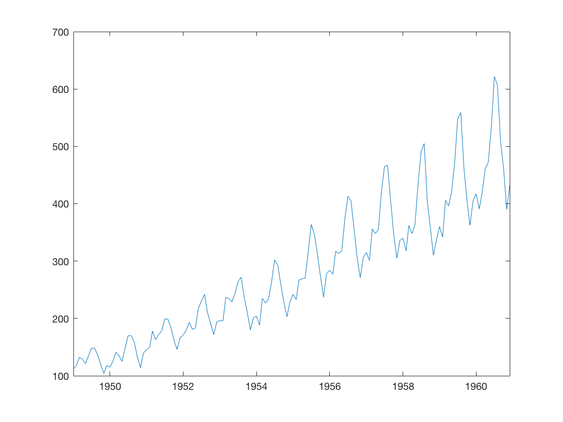
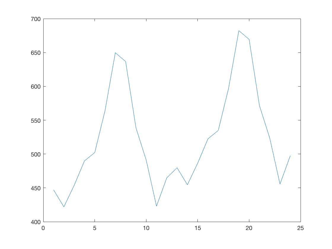
b) Fit an ARIMA model and predict 2 years (24 months).
model = arima('Constant',0,'D',1,'Seasonality',12,...
    'MALags',1,'SMALags',12);
est_model = estimate(model, air.AIR);
[yF, yMSE] = forecast(est_model, 24, 'Y0', air.AIR);
plot(yF);
    ARIMA(0,1,1) Model Seasonally Integrated with Seasonal MA(12):
    ---------------------------------------------------------------
    Conditional Probability Distribution: Gaussian

                                  Standard          t
     Parameter       Value          Error       Statistic
    -----------   -----------   ------------   -----------
     Constant              0         Fixed          Fixed
        MA{1}      -0.309349     0.0619375       -4.99454
      SMA{12}      -0.112821      0.082419       -1.36887
     Variance        123.282       12.5426        9.82908
9 Model Evaluation & Selection
9.1 Evaluate the accuracy of regression models.
a) Evaluation on training data.
train = readtable('boston_train.xlsx');
test = readtable('boston_test.xlsx');
x_train = train;
x_train.Target = [];
y_train = train.Target;
x_test = test;
x_test.Target = [];
y_test = test.Target;
rng(29);
rfMod = fitrensemble(table2array(x_train), y_train, 'Method', 'bag');
predictions = predict(rfMod, table2array(x_train));
r2_rf = 1 - ( (sum((y_train - predictions) .^ 2)) / (sum((y_train - mean(y_train)) .^ 2)) );
fprintf('Random forest regression model r^2 score (coefficient of determination): %.3f\n', r2_rf);
Random forest regression model r^2 score (coefficient of determination): 0.930readtable() | rng() | table2array() | fitrensemble() | predict() | mean() | sum() | fprintf()
b) Evaluation on testing data.
predictions = predict(rfMod, table2array(x_test));
r2_rf = 1 - ( (sum((y_test - predictions) .^ 2)) / (sum((y_test - mean(y_test)) .^ 2)) );
fprintf('Random forest regression model r^2 score (coefficient of determination): %.3f\n', r2_rf);
Random forest regression model r^2 score (coefficient of determination): 0.867predict() | mean() | sum() | fprintf()
9.2 Evaluate the accuracy of classification models.
a) Evaluation on training data.
train = readtable('digits_train.xlsx');
test = readtable('digits_test.xlsx');
x_train = train;
x_train.Target = [];
y_train = train.Target;
x_test = test;
x_test.Target = [];
y_test = test.Target;
rng(29);
rfMod = fitrensemble(table2array(x_train), y_train, 'Method', 'bag');
predY = predict(rfMod, table2array(x_train));
predY = round(predY);
Results = zeros(size(train,1),1);
for i = 1:size(Results,1)
    if (predY(i) == y_train(i))
        Results(i) = 1;
    else
        Results(i) = 0;
    end
end
accuracy_rf = (1/size(x_train,1)) * sum(Results);
fprintf('Random forest model accuracy:  %.3f\n', accuracy_rf);
Random forest model accuracy: 0.692readtable() | rng() | table2array() | fitrensemble() | predict() | round() | size() | zeros() | sum() | fprintf()
b) Evaluation on testing data.
predY = predict(rfMod, table2array(x_test));
predY = round(predY);
Results = zeros(size(test,1),1);
for i = 1:size(Results,1)
    if (predY(i) == y_test(i))
        Results(i) = 1;
    else
        Results(i) = 0;
    end
end
accuracy_rf = (1/size(x_test,1)) * sum(Results);
fprintf('Random forest model accuracy:  %.3f\n', accuracy_rf);
Random forest model accuracy: 0.526predict() | round() | size() | zeros() | sum() | fprintf()
Appendix
1 Built-in MATLAB Data Types
Numeric types
- Integer and floating-point data
Characters and strings
- Text in character arrays and string arrays
Tables
- Arrays in tabular form whose named columns can have different types
Structures
- Arrays with named fields that can contain data of varying types and sizes
Cell arrays
- Arrays that can contain data of varying types and sizes
Alphabetical Index
Note, from the MathWorks website: "MATLAB is an abbreviation for "matrix laboratory." While other programming languages mostly work with numbers one at a time, MATLAB® is designed to operate primarily on whole matrices and arrays. All MATLAB variables are multidimensional arrays, no matter what type of data."
Matrix
A matrix is a two-dimensional array often used for linear algebra operations. Please see the following example of matrix creation and access:
my_matrix = [1 2 3; 4 5 6; 7 8 9]
disp(my_matrix(2,2));
5