Python Tutorial
Welcome to the Python tutorial version of Data Science Rosetta Stone. Before beginning this tutorial, please check to make sure you have Python 3.5.2 installed (this is not required, but this was the release used to generate the following examples). Also, the following Python packages are used throughout this tutorial. You may not need all of the following packages to fit your specific needs, but they are listed below, and also in Appendix Section 2 with more detail, for your information:
- pandas (0.20.2)
- NumPy (1.12.1)
- Matplotlib.PyPlot
- seaborn (0.7.1)
- re (2.2.1)
- decimal (1.70)
- sklearn (0.18.2)
- statsmodels.api
- xgboost (0.6)
- pyclustering
- PyFlux (0.4.15)
- FBProphet
To install Python packages, you need to run the following in the command line/terminal of your computer:
pip install package_name
# or #
conda install package_nameNote: In Python, comments are indicated in code with a “#” character, and arrays and matrices are zero-indexed.
Now let’s get started! First, you need to import several very important Python packages for data manipulation and scientific computing. The pandas package is useful for data manipulation and the NumPy package is useful for scientific computing.
import pandas as pd
import numpy as np
1 Reading in Data and Basic Statistical Functions
1.1 Read in the data.
The following demonstrate importing data into Python given 3 different file formats. The pandas package is able to read all 3 formats, as well as many others, using Python IO tools.
a) Read the data in as a .csv file.
student = pd.read_csv('/Users/class.csv')b) Read the data in as a .xls file.
# Notice you must specify the file location, as well as the name of the sheet
# of the .xls file you want to import
student_xls = pd.read_excel(open('/Users/class.xls', 'rb'),
                            sheetname='class')
c) Read the data in as a .json file.
student_json = pd.read_json('/Users/class.json')1.2 Find the dimensions of the data set.
The dimensions of a DataFrame in Python are known as an attribute of the object. Therefore, you can state the data name followed by .shape to return the dimensions of the data, with the first integer indicating the number of rows and the second indicating the number of columns.
print(student.shape)## (19, 5)1.3 Find basic information about the data set.
Information about a DataFrame is available by calling the info() function on the data.
print(student.info())## <class 'pandas.core.frame.DataFrame'>
## RangeIndex: 19 entries, 0 to 18
## Data columns (total 5 columns):
## Name 19 non-null object
## Sex 19 non-null object
## Age 19 non-null int64
## Height 19 non-null float64
## Weight 19 non-null float64
## dtypes: float64(2), int64(1), object(2)
## memory usage: 840.0+ bytes
## None1.4 Look at the first 5 (last 5) observations.
The first 5 observations of a DataFrame are available by calling the head() function on the data. By default, head() returns 5 observations. To return the first n observations, pass the integer n into the function. The tail() function is analogous and returns the last observations.
print(student.head())## Name Sex Age Height Weight
## 0 Alfred M 14 69.0 112.5
## 1 Alice F 13 56.5 84.0
## 2 Barbara F 13 65.3 98.0
## 3 Carol F 14 62.8 102.5
## 4 Henry M 14 63.5 102.51.5 Calculate means of numeric variables.
The means of numeric variables of a DataFrame are available by calling the mean() function on the data.
print(student.mean())## Age 13.315789
## Height 62.336842
## Weight 100.026316
## dtype: float641.6 Compute summary statistics of the data set.
Summary statistics of a DataFrame are available by calling the describe() function on the data.
print(student.describe())## Age Height Weight
## count 19.000000 19.000000 19.000000
## mean 13.315789 62.336842 100.026316
## std 1.492672 5.127075 22.773933
## min 11.000000 51.300000 50.500000
## 25% 12.000000 58.250000 84.250000
## 50% 13.000000 62.800000 99.500000
## 75% 14.500000 65.900000 112.250000
## max 16.000000 72.000000 150.0000001.7 Descriptive statistics functions applied to variables of the data set.
# Notice the subsetting of student with [] and the name of the variable in
# quotes ("")
print(student["Weight"].std())
## 22.773933493879046print(student["Weight"].sum())## 1900.5print(student["Weight"].count())## 19print(student["Weight"].max())## 150.0print(student["Weight"].min())## 50.5print(student["Weight"].median())## 99.51.8 Produce a one-way table to describe the frequency of a variable.
a) Produce a one-way table of a discrete variable.
# columns = "count" indicates to make the descriptive portion of the table
# the counts of each level of the index variable
print(pd.crosstab(index=student["Age"], columns="count"))
## col_0 count
## Age
## 11 2
## 12 5
## 13 3
## 14 4
## 15 4
## 16 1b) Produce a one-way table of a categorical variable.
print(pd.crosstab(index=student["Sex"], columns="count"))## col_0 count
## Sex
## F 9
## M 101.9 Produce a two-way table to describe the frequency of two categorical or discrete variables.
# Notice the specification of a variable for the columns argument, instead
# of "count"
print(pd.crosstab(index=student["Age"], columns=student["Sex"]))
## Sex F M
## Age
## 11 1 1
## 12 2 3
## 13 2 1
## 14 2 2
## 15 2 2
## 16 0 11.10 Select a subset of the data that meets a certain criterion.
females = student.query('Sex == "F"')
print(females.head())
## Name Sex Age Height Weight
## 1 Alice F 13 56.5 84.0
## 2 Barbara F 13 65.3 98.0
## 3 Carol F 14 62.8 102.5
## 6 Jane F 12 59.8 84.5
## 7 Janet F 15 62.5 112.51.11 Determine the correlation between two continuous variables.
# axis = 1 option indicates to concatenate column-wise
height_weight = pd.concat([student["Height"], student["Weight"]], axis = 1)
print(height_weight.corr(method = "pearson"))
## Height Weight
## Height 1.000000 0.877785
## Weight 0.877785 1.0000002 Basic Graphing and Plotting Functions
The Matplotlib PyPlot package is a standard Python package to use for plotting. For more information on other Python plotting packages, please see the Appendix Section 2.
import matplotlib.pyplot as plt2.1 Visualize a single continuous variable by producing a histogram.
plt.hist(student["Weight"], bins=[40,60,80,100,120,140,160])
plt.xlabel('Weight')
plt.ylabel('Frequency')
plt.show()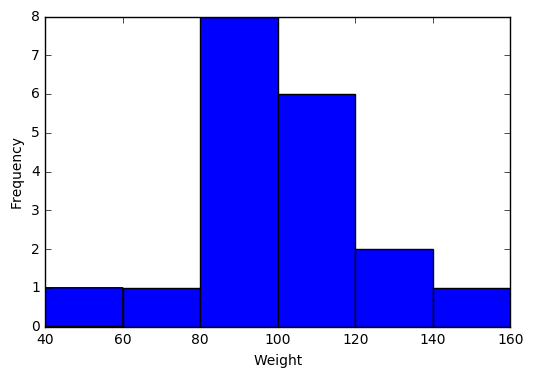
2.2 Visualize a single continuous variable by producing a boxplot.
# showmeans=True tells Python to plot the mean of the variable on the boxplot
plt.boxplot(student["Weight"], showmeans=True)

# prevents Python from printing a "1" at the bottom of the boxplot
plt.xticks([])

plt.ylabel('Weight')
plt.show()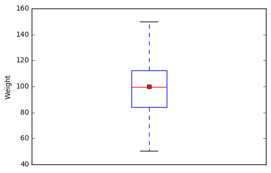
2.3 Visualize two continuous variables by producing a scatterplot.
# Notice here you specify the x variable, followed by the y variable
plt.scatter(student["Height"], student["Weight"])
plt.xlabel("Height")
plt.ylabel("Weight")
plt.show()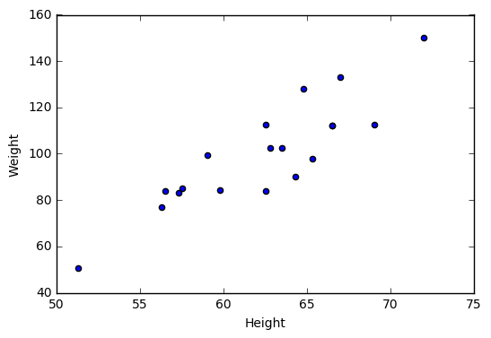
2.4 Visualize a relationship between two continuous variables by producing a scatterplot and a plotted line of best fit.
x = student["Height"]
y = student["Weight"]

# np.polyfit() models Weight as a function of Height and returns the
# parameters
m, b = np.polyfit(x, y, 1)
plt.scatter(x, y)

# plt.text() prints the equation of the line of best fit, with the first two
# arguments specifying the x and y locations of the text, respectively
# "%f" indicates to print a floating point number, that is specified following
# the string and a "%" character
plt.text(51, 140, "Line: y = %f x + %f"% (m,b))
plt.plot(x, m*x + b)
plt.xlabel("Height")
plt.ylabel("Weight")
plt.show()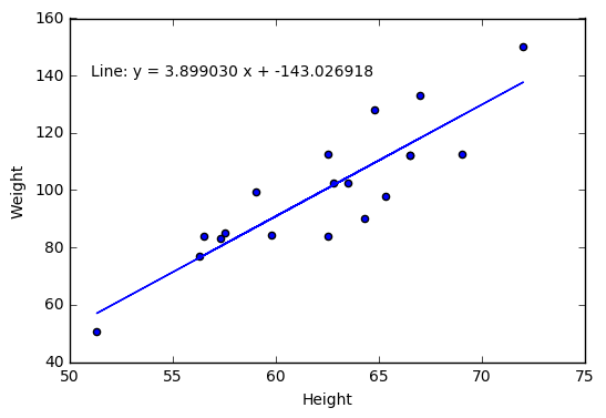
2.5 Visualize a categorical variable by producing a bar chart.
# Get the counts of Sex
counts = pd.crosstab(index=student["Sex"], columns="count")

# len() returns the number of categories of Sex (2)
# np.arange() creates a vector of the specified length
num = np.arange(len(counts))

# alpha = 0.5 changes the transparency of the bars
plt.bar(num, counts["count"], align='center', alpha=0.5)

# Set the xticks to be the indices of counts
plt.xticks(num, counts.index)
plt.xlabel("Sex")
plt.ylabel("Frequency")
plt.show()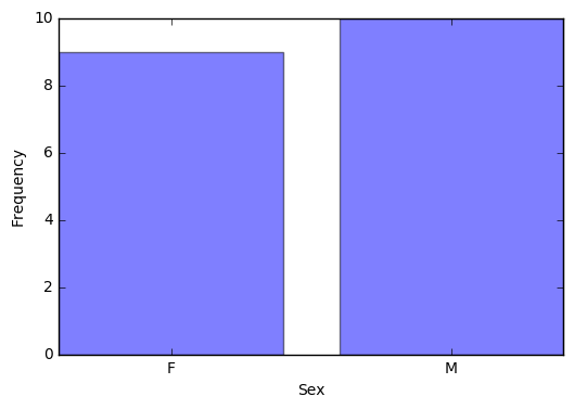
2.6 Visualize a continuous variable, grouped by a categorical variable, by producing side-by-side boxplots.
a) Simple side-by-side boxplot without color.
# Subset data set to return only female weights, and then only male weights
Weight_F = np.array(student.query('Sex == "F"')["Weight"])
Weight_M = np.array(student.query('Sex == "M"')["Weight"])
Weights = [Weight_F, Weight_M]

# PyPlot automatically plots the two weights side-by-side since Weights
# is a 2D array
plt.boxplot(Weights, showmeans=True, labels=('F', 'M'))
plt.xlabel('Sex')
plt.ylabel('Weight')
plt.show()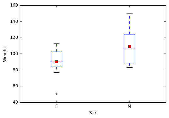
b) More advanced side-by-side boxplot with color.
import seaborn as sns
sns.boxplot(x="Sex", y="Weight", hue="Sex", data = student, showmeans=True)
sns.plt.show()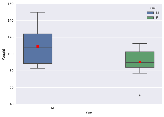
3 Basic Data Wrangling and Manipulation
3.1 Create a new variable in a data set as a function of existing variables in the data set.
# Notice here how you can create the BMI column in the data set
# just by naming it
student["BMI"] = student["Weight"] / student["Height"]**2 * 703
print(student.head())
## Name Sex Age Height Weight BMI
## 0 Alfred M 14 69.0 112.5 16.611531
## 1 Alice F 13 56.5 84.0 18.498551
## 2 Barbara F 13 65.3 98.0 16.156788
## 3 Carol F 14 62.8 102.5 18.270898
## 4 Henry M 14 63.5 102.5 17.8702963.2 Create a new variable in a data set using if/else logic of existing variables in the data set.
# Notice the use of the np.where() function for a single condition
student["BMI Class"] = np.where(student["BMI"] < 19.0, "Underweight",
                                "Healthy")
print(student.head())
## Name Sex Age Height Weight BMI BMI Class
## 0 Alfred M 14 69.0 112.5 16.611531 Underweight
## 1 Alice F 13 56.5 84.0 18.498551 Underweight
## 2 Barbara F 13 65.3 98.0 16.156788 Underweight
## 3 Carol F 14 62.8 102.5 18.270898 Underweight
## 4 Henry M 14 63.5 102.5 17.870296 Underweight3.3 Create new variables in a data set using mathematical functions applied to existing variables in the data set.
Using the np.log(), np.exp(), np.sqrt(), np.where(), and np.abs() functions.
student["LogWeight"] = np.log(student["Weight"])
student["ExpAge"] = np.exp(student["Age"])
student["SqrtHeight"] = np.sqrt(student["Height"])
student["BMI Neg"] = np.where(student["BMI"] < 19.0, -student["BMI"],
                              student["BMI"])
student["BMI Pos"] = np.abs(student["BMI Neg"])

# Create a Boolean variable
student["BMI Check"] = (student["BMI Pos"] == student["BMI"])
## Name Sex Age Height Weight BMI BMI Class LogWeight \
## 0 Alfred M 14 69.0 112.5 16.611531 Underweight 4.722953
## 1 Alice F 13 56.5 84.0 18.498551 Underweight 4.430817
## 2 Barbara F 13 65.3 98.0 16.156788 Underweight 4.584967
## 3 Carol F 14 62.8 102.5 18.270898 Underweight 4.629863
## 4 Henry M 14 63.5 102.5 17.870296 Underweight 4.629863
##
## ExpAge SqrtHeight BMI Neg BMI Pos BMI Check
## 0 1.202604e+06 8.306624 -16.611531 16.611531 True
## 1 4.424134e+05 7.516648 -18.498551 18.498551 True
## 2 4.424134e+05 8.080842 -16.156788 16.156788 True
## 3 1.202604e+06 7.924645 -18.270898 18.270898 True
## 4 1.202604e+06 7.968689 -17.870296 17.870296 True3.4 Drop variables from a data set.
# axis = 1 indicates to drop columns instead of rows
student = student.drop(["LogWeight", "ExpAge", "SqrtHeight", "BMI Neg",
                        "BMI Pos", "BMI Check"], axis = 1)
print(student.head())
## Name Sex Age Height Weight BMI BMI Class
## 0 Alfred M 14 69.0 112.5 16.611531 Underweight
## 1 Alice F 13 56.5 84.0 18.498551 Underweight
## 2 Barbara F 13 65.3 98.0 16.156788 Underweight
## 3 Carol F 14 62.8 102.5 18.270898 Underweight
## 4 Henry M 14 63.5 102.5 17.870296 Underweight3.5 Sort a data set by a variable.
a) Sort data set by a continuous variable.
# Notice kind="mergesort" which indicates to use a stable sorting
# algorithm
student = student.sort_values(by="Age", kind="mergesort")
print(student.head())
## Name Sex Age Height Weight BMI BMI Class
## 10 Joyce F 11 51.3 50.5 13.490001 Underweight
## 17 Thomas M 11 57.5 85.0 18.073346 Underweight
## 5 James M 12 57.3 83.0 17.771504 Underweight
## 6 Jane F 12 59.8 84.5 16.611531 Underweight
## 9 John M 12 59.0 99.5 20.094369 Healthyb) Sort data set by a categorical variable.
student = student.sort_values(by="Sex", kind="mergesort")
# Notice that the data is now sorted first by Sex and then within Sex by Age
print(student.head())
## Name Sex Age Height Weight BMI BMI Class
## 10 Joyce F 11 51.3 50.5 13.490001 Underweight
## 6 Jane F 12 59.8 84.5 16.611531 Underweight
## 12 Louise F 12 56.3 77.0 17.077695 Underweight
## 1 Alice F 13 56.5 84.0 18.498551 Underweight
## 2 Barbara F 13 65.3 98.0 16.156788 Underweight3.6 Compute descriptive statistics of continuous variables, grouped by a categorical variable.
print(student.groupby(by="Sex").mean())## Age Height Weight BMI
## Sex
## F 13.222222 60.588889 90.111111 17.051039
## M 13.400000 63.910000 108.950000 18.5942433.7 Add a new row to the bottom of a data set.
# Look at the tail of the data currently
print(student.tail())
## Name Sex Age Height Weight BMI BMI Class
## 0 Alfred M 14 69.0 112.5 16.611531 Underweight
## 4 Henry M 14 63.5 102.5 17.870296 Underweight
## 16 Ronald M 15 67.0 133.0 20.828470 Healthy
## 18 William M 15 66.5 112.0 17.804511 Underweight
## 14 Philip M 16 72.0 150.0 20.341435 Healthystudent = student.append({'Name':'Jane', 'Sex':'F', 'Age':14, 'Height':56.3,
'Weight':77.0, 'BMI':17.077695,
'BMI Class': 'Underweight'},
ignore_index=True)
# Notice the change in the indices because of the ignore_index=True option
# which allows for a Series, or one-dimensional DataFrame, to be appended
# to an existing DataFrame ## Name Sex Age Height Weight BMI BMI Class
## 15 Henry M 14 63.5 102.5 17.870296 Underweight
## 16 Ronald M 15 67.0 133.0 20.828470 Healthy
## 17 William M 15 66.5 112.0 17.804511 Underweight
## 18 Philip M 16 72.0 150.0 20.341435 Healthy
## 19 Jane F 14 56.3 77.0 17.077695 Underweight3.8 Create a user-defined function and apply it to a variable in the data set to create a new variable in the data set.
def toKG(lb):
    return (0.45359237 * lb)

student["Weight KG"] = student["Weight"].apply(toKG)
print(student.head())
## Name Sex Age Height Weight BMI BMI Class Weight KG
## 0 Joyce F 11 51.3 50.5 13.490001 Underweight 22.906415
## 1 Jane F 12 59.8 84.5 16.611531 Underweight 38.328555
## 2 Louise F 12 56.3 77.0 17.077695 Underweight 34.926612
## 3 Alice F 13 56.5 84.0 18.498551 Underweight 38.101759
## 4 Barbara F 13 65.3 98.0 16.156788 Underweight 44.452052apply() | user-defined functions
4 More Advanced Data Wrangling
4.1 Drop observations with missing information.
# Notice the use of the fish data set because it has some missing
# observations
fish = pd.read_csv('/Users/fish.csv')

# First sort by Weight, requesting those with NA for Weight first
fish = fish.sort_values(by='Weight', kind='mergesort', na_position='first')
print(fish.head())
## Species Weight Length1 Length2 Length3 Height Width
## 13 Bream NaN 29.5 32.0 37.3 13.9129 5.0728
## 40 Roach 0.0 19.0 20.5 22.8 6.4752 3.3516
## 72 Perch 5.9 7.5 8.4 8.8 2.1120 1.4080
## 145 Smelt 6.7 9.3 9.8 10.8 1.7388 1.0476
## 147 Smelt 7.0 10.1 10.6 11.6 1.7284 1.1484–
new_fish = fish.dropna()
print(new_fish.head())
## Species Weight Length1 Length2 Length3 Height Width
## 40 Roach 0.0 19.0 20.5 22.8 6.4752 3.3516
## 72 Perch 5.9 7.5 8.4 8.8 2.1120 1.4080
## 145 Smelt 6.7 9.3 9.8 10.8 1.7388 1.0476
## 147 Smelt 7.0 10.1 10.6 11.6 1.7284 1.1484
## 146 Smelt 7.5 10.0 10.5 11.6 1.9720 1.16004.2 Merge two data sets together on a common variable.
a) First, select specific columns of a data set to create two smaller data sets.
# Notice the use of the student data set again, however we want to reload it
# without the changes we've made previously
student = pd.read_csv('/Users/class.csv')
student1 = pd.concat([student["Name"], student["Sex"], student["Age"]],
                    axis = 1)
print(student1.head())
## Name Sex Age
## 0 Alfred M 14
## 1 Alice F 13
## 2 Barbara F 13
## 3 Carol F 14
## 4 Henry M 14–
student2 = pd.concat([student["Name"], student["Height"], student["Weight"]],
                    axis = 1)
print(student2.head())
## Name Height Weight
## 0 Alfred 69.0 112.5
## 1 Alice 56.5 84.0
## 2 Barbara 65.3 98.0
## 3 Carol 62.8 102.5
## 4 Henry 63.5 102.5b) Second, we want to merge the two smaller data sets on the common variable.
new = pd.merge(student1, student2, on="Name")
print(new.head())
## Name Sex Age Height Weight
## 0 Alfred M 14 69.0 112.5
## 1 Alice F 13 56.5 84.0
## 2 Barbara F 13 65.3 98.0
## 3 Carol F 14 62.8 102.5
## 4 Henry M 14 63.5 102.5c) Finally, we want to check to see if the merged data set is the same as the original data set.
print(student.equals(new))## True4.3 Merge two data sets together by index number only.
a) First, select specific columns of a data set to create two smaller data sets.
newstudent1 = pd.concat([student["Name"], student["Sex"], student["Age"]],
                        axis = 1)
print(newstudent1.head())
## Name Sex Age
## 0 Alfred M 14
## 1 Alice F 13
## 2 Barbara F 13
## 3 Carol F 14
## 4 Henry M 14–
newstudent2 = pd.concat([student["Height"], student["Weight"]], axis = 1)
print(newstudent2.head())
## Height Weight
## 0 69.0 112.5
## 1 56.5 84.0
## 2 65.3 98.0
## 3 62.8 102.5
## 4 63.5 102.5b) Second, we want to join the two smaller data sets.
new2 = newstudent1.join(newstudent2)
print(new2.head())
## Name Sex Age Height Weight
## 0 Alfred M 14 69.0 112.5
## 1 Alice F 13 56.5 84.0
## 2 Barbara F 13 65.3 98.0
## 3 Carol F 14 62.8 102.5
## 4 Henry M 14 63.5 102.5c) Finally, we want to check to see if the joined data set is the same as the original data set.
print(student.equals(new2))## True4.4 Create a pivot table to summarize information about a data set.
# Notice we are using a new data set that needs to be read into the
# environment
price = pd.read_csv('/Users/price.csv')

# The following code is used to remove the "," and "$" characters from
# the ACTUAL colum so that the values can be summed
from re import sub
from decimal import Decimal
def trim_money(money):
    return(float(Decimal(sub(r'[^\d.]', '', money))))

price["REVENUE"] = price["ACTUAL"].apply(trim_money)
table = pd.pivot_table(price, index=["COUNTRY", "STATE", "PRODTYPE",
                                     "PRODUCT"], values="REVENUE",
                       aggfunc=np.sum)
print(table.head())
## REVENUE
## COUNTRY STATE PRODTYPE PRODUCT
## Canada British Columbia FURNITURE BED 197706.6
## SOFA 216282.6
## OFFICE CHAIR 200905.2
## DESK 186262.2
## Ontario FURNITURE BED 194493.6Note: pd.pivot_table() is similar to the pd.pivot() function.
4.5 Return all unique values from a text variable.
print(np.unique(price["STATE"]))## ['Baja California Norte' 'British Columbia' 'California' 'Campeche'
## 'Colorado' 'Florida' 'Illinois' 'Michoacan' 'New York' 'North Carolina'
## 'Nuevo Leon' 'Ontario' 'Quebec' 'Saskatchewan' 'Texas' 'Washington']The following sections focus on the Python sklearn package. Also, in the following sections, several data set will be used more than once for prediction and modeling. Often, they will be re-read into the environment so we are always going back to the original, raw data.
5 Preparation & Basic Regression
5.1 Pre-process a data set using principal component analysis.
# Notice we are using a new data set that needs to be read into the
# environment
iris = pd.read_csv('/Users/iris.csv')
features = iris.drop(["Target"], axis = 1)

from sklearn import preprocessing
features_scaled = preprocessing.scale(features.as_matrix())

from sklearn.decomposition import PCA

pca = PCA(n_components = 4)
pca = pca.fit(features_scaled)
print(np.transpose(pca.components_))
## [[ 0.52237162 0.37231836 -0.72101681 -0.26199559]
## [-0.26335492 0.92555649 0.24203288 0.12413481]
## [ 0.58125401 0.02109478 0.14089226 0.80115427]
## [ 0.56561105 0.06541577 0.6338014 -0.52354627]]5.2 Split data into training and testing data and export as a .csv file.
from sklearn.model_selection import train_test_split

target = iris["Target"]

# The following code splits the iris data set into 70% train and 30% test
X_train, X_test, Y_train, Y_test = train_test_split(features, target,
                                                    test_size = 0.3,
                                                    random_state = 29)
train_x = pd.DataFrame(X_train)
train_y = pd.DataFrame(Y_train)
test_x = pd.DataFrame(X_test)
test_y = pd.DataFrame(Y_test)

train = pd.concat([train_x, train_y], axis = 1)
test = pd.concat([test_x, test_y], axis = 1)

train.to_csv('/Users/iris_train_Python.csv', index = False)
test.to_csv('/Users/iris_test_Python.csv', index = False)5.3 Fit a logistic regression model.
# Notice we are using a new data set that needs to be read into the
# environment
tips = pd.read_csv('/Users/tips.csv')

# The following code is used to determine if the individual left more
# than a 15% tip
tips["fifteen"] = 0.15 * tips["total_bill"]
tips["greater15"] = np.where(tips["tip"] > tips["fifteen"], 1, 0)

import statsmodels.api as sm

# Notice the syntax of greater15 as a function of total_bill
logreg = sm.formula.glm("greater15 ~ total_bill",
                       family=sm.families.Binomial(),
                       data=tips).fit()
print(logreg.summary())
##                  Generalized Linear Model Regression Results
## ==============================================================================
## Dep. Variable:              greater15   No. Observations:                  244
## Model:                            GLM   Df Residuals:                      242
## Model Family:                Binomial   Df Model:                            1
## Link Function:                  logit   Scale:                             1.0
## Method:                          IRLS   Log-Likelihood:                -156.87
## Date:                Wed, 05 Jul 2017   Deviance:                       313.74
## Time:                        13:50:25   Pearson chi2:                     247.
## No. Iterations:                     4
## ==============================================================================
##                  coef    std err          z      P>|z|      [0.025      0.975]
## ------------------------------------------------------------------------------
## Intercept      1.6477      0.355      4.646      0.000       0.953       2.343
## total_bill    -0.0725      0.017     -4.319      0.000      -0.105      -0.040
## ==============================================================================
A logistic regression model can be implemented using sklearn, however statsmodels.api provides a helpful summary about the model, so it is preferable for this example.
5.4 Fit a linear regression model.
# Fit a linear regression model of tip by total_bill
from sklearn.linear_model import LinearRegression

# If your data has one feature, you need to reshape the 1D array
linreg = LinearRegression()
linreg.fit(tips["total_bill"].values.reshape(-1,1), tips["tip"])
print(linreg.coef_)
print(linreg.intercept_)
## [ 0.10502452]
## 0.9202696135556 Supervised Machine Learning
6.1 Fit a logistic regression model on training data and assess against testing data.
a) Fit a logistic regression model on training data.
# Notice we are using new data sets that need to be read into the environment
train = pd.read_csv('/Users/tips_train.csv')
test = pd.read_csv('/Users/tips_test.csv')

train["fifteen"] = 0.15 * train["total_bill"]
train["greater15"] = np.where(train["tip"] > train["fifteen"], 1, 0)
test["fifteen"] = 0.15 * test["total_bill"]
test["greater15"] = np.where(test["tip"] > test["fifteen"], 1, 0)

logreg = sm.formula.glm("greater15 ~ total_bill",
                       family=sm.families.Binomial(),
                       data=train).fit()
print(logreg.summary())
##                  Generalized Linear Model Regression Results
## ==============================================================================
## Dep. Variable:              greater15   No. Observations:                  195
## Model:                            GLM   Df Residuals:                      193
## Model Family:                Binomial   Df Model:                            1
## Link Function:                  logit   Scale:                             1.0
## Method:                          IRLS   Log-Likelihood:                -125.29
## Date:                Wed, 05 Jul 2017   Deviance:                       250.58
## Time:                        13:50:28   Pearson chi2:                     197.
## No. Iterations:                     4
## ==============================================================================
##                  coef    std err          z      P>|z|      [0.025      0.975]
## ------------------------------------------------------------------------------
## Intercept      1.6461      0.395      4.172      0.000       0.873       2.420
## total_bill    -0.0706      0.018     -3.820      0.000      -0.107      -0.034
## ==============================================================================
b) Assess the model against the testing data.
# Prediction on testing data
predictions = logreg.predict(test["total_bill"])
predY = np.where(predictions < 0.5, 0, 1)

# If the prediction probability is less than 0.5, classify this as a 0
# and otherwise classify as a 1.  This isn't the best method -- a better
# method would be randomly assigning a 0 or 1 when a probability of 0.5
# occurrs, but this insures that results are consistent

# Determine how many were correctly classified
Results = np.where(predY == test["greater15"], "Correct", "Wrong")
print(pd.crosstab(index=Results, columns="count"))
## col_0    count
## row_0
## Correct     34
## Wrong       15
A logistic regression model can be implemented using sklearn, however statsmodels.api provides a helpful summary about the model, so it is preferable for this example.
6.2 Fit a linear regression model on training data and assess against testing data.
a) Fit a linear regression model on training data.
# Notice we are using new data sets that need to be read into the environment
train = pd.read_csv('/Users/boston_train.csv')
test = pd.read_csv('/Users/boston_test.csv')

# Fit a linear regression model
linreg = LinearRegression()
linreg.fit(train.drop(["Target"], axis = 1), train["Target"])
print(linreg.coef_)
print(linreg.intercept_)
## [ -8.56336900e-02 4.60343577e-02 3.64131905e-02 3.24796064e+00
## -1.48729382e+01 3.57686873e+00 -8.70316831e-03 -1.36890461e+00
## 3.13120107e-01 -1.28815611e-02 -9.76900124e-01 1.13257346e-02
## -5.26715028e-01]
## 36.1081957809b) Assess the model against the testing data.
# Prediction on testing data
prediction = pd.DataFrame()
prediction["predY"] = linreg.predict(test.drop(["Target"], axis = 1))

# Determine mean squared error
prediction["sq_diff"] = (prediction["predY"] - test["Target"])**2
print(np.mean(prediction["sq_diff"]))
## 17.7713079588916726.3 Fit a decision tree model on training data and assess against testing data.
a) Fit a decision tree classification model.
i) Fit a decision tree classification model on training data and determine variable importance.
# Notice we are using new data sets that need to be read into the environment
train = pd.read_csv('/Users/breastcancer_train.csv')
test = pd.read_csv('/Users/breastcancer_test.csv')

from sklearn.tree import DecisionTreeClassifier

# random_state is used to specify a seed for a random integer so that the
# results are reproducible
treeMod = DecisionTreeClassifier(random_state=29)
treeMod.fit(train.drop(["Target"], axis = 1), train["Target"])

# Determine variable importance
var_import = treeMod.feature_importances_
var_import = pd.DataFrame(var_import)
var_import = var_import.rename(columns = {0:'Importance'})
var_import = var_import.sort_values(by="Importance", kind = "mergesort",
                                    ascending = False)
print(var_import.head())
## Importance
## 23 0.692681
## 27 0.158395
## 21 0.044384
## 11 0.029572
## 24 0.020485ii) Assess the model against the testing data.
# Prediction on testing data
predY = treeMod.predict(test.drop(["Target"], axis = 1))

# Determine how many were correctly classified
Results = np.where(test["Target"] == predY, "Correct", "Wrong")
print(pd.crosstab(index=Results, columns="count"))
## col_0 count
## row_0
## Correct 161
## Wrong 10b) Fit a decision tree regression model.
i) Fit a decision tree regression model on training data and determine variable importance.
train = pd.read_csv('/Users/boston_train.csv')
test = pd.read_csv('/Users/boston_test.csv')

from sklearn.tree import DecisionTreeRegressor

treeMod = DecisionTreeRegressor(random_state=29)
treeMod.fit(train.drop(["Target"], axis = 1), train["Target"])

# Determine variable importance
var_import = treeMod.feature_importances_
var_import = pd.DataFrame(var_import)
var_import = var_import.rename(columns = {0:'Importance'})
var_import = var_import.sort_values(by="Importance", kind = "mergesort",
                                    ascending = False)
print(var_import.head())
## Importance
## 5 0.573257
## 12 0.203677
## 7 0.103939
## 4 0.041467
## 0 0.033798ii) Assess the model against the testing data.
# Prediction on testing data
prediction = pd.DataFrame()
prediction["predY"] = treeMod.predict(test.drop(["Target"], axis = 1))

# Determine mean squared error
prediction["sq_diff"] = (prediction["predY"] - test["Target"])**2
print(np.mean(prediction["sq_diff"]))
## 23.8668421052631576.4 Fit a random forest model on training data and assess against testing data.
a) Fit a random forest classification model.
i) Fit a random forest classification model on training data and determine variable importance.
train = pd.read_csv('/Users/breastcancer_train.csv')
test = pd.read_csv('/Users/breastcancer_test.csv')

from sklearn.ensemble import RandomForestClassifier

rfMod = RandomForestClassifier(random_state=29)
rfMod.fit(train.drop(["Target"], axis = 1), train["Target"])

# Determine variable importance
var_import = rfMod.feature_importances_
var_import = pd.DataFrame(var_import)
var_import = var_import.rename(columns = {0:'Importance'})
var_import = var_import.sort_values(by="Importance", kind = "mergesort",
                                    ascending = False)
print(var_import.head())
## Importance
## 27 0.271730
## 13 0.120096
## 23 0.101971
## 20 0.076891
## 6 0.066836ii) Assess the model against the testing data.
# Prediction on testing data
predY = rfMod.predict(test.drop(["Target"], axis = 1))

# Determine how many were correctly classified
Results = np.where(test["Target"] == predY, "Correct", "Wrong")
print(pd.crosstab(index=Results, columns="count"))
## col_0 count
## row_0
## Correct 165
## Wrong 6b) Fit a random forest regression model.
i) Fit a random forest regression model on training data and determine variable importance.
train = pd.read_csv('/Users/boston_train.csv')
test = pd.read_csv('/Users/boston_test.csv')
from sklearn.ensemble import RandomForestRegressor
rfMod = RandomForestRegressor(random_state=29)
rfMod.fit(train.drop(["Target"], axis = 1), train["Target"])
# Determine variable importance
var_import = rfMod.feature_importances_
var_import = pd.DataFrame(var_import)
var_import = var_import.rename(columns = {0:'Importance'})
var_import = var_import.sort_values(by="Importance", kind = "mergesort",
ascending = False)
print(var_import.head())## Importance
## 5 0.412012
## 12 0.392795
## 7 0.079462
## 0 0.041911
## 9 0.016374ii) Assess the model against the testing data.
# Prediction on testing data
prediction = pd.DataFrame()
prediction["predY"] = rfMod.predict(test.drop(["Target"], axis = 1))
# Determine mean squared error
prediction["sq_diff"] = (test["Target"] - prediction["predY"])**2
print(prediction["sq_diff"].mean())## 13.250326315789486.5 Fit a gradient boosting model on training data and assess against testing data.
a) Fit a gradient boosting classification model.
i) Fit a gradient boosting classification model on training data and determine variable importance.
train = pd.read_csv('/Users/breastcancer_train.csv')
test = pd.read_csv('/Users/breastcancer_test.csv')
from sklearn.ensemble import GradientBoostingClassifier
# n_estimators = total number of trees to fit which is analogous to the
# number of iterations
# learning_rate = shrinkage or step-size reduction, where a lower
# learning rate requires more iterations
gbMod = GradientBoostingClassifier(random_state = 29, learning_rate = .01,
n_estimators = 2500)
gbMod.fit(train.drop(["Target"], axis = 1), train["Target"])
# Determine variable importance
var_import = gbMod.feature_importances_
var_import = pd.DataFrame(var_import)
var_import = var_import.rename(columns = {0:'Importance'})
var_import = var_import.sort_values(by="Importance", kind = "mergesort",
ascending = False)
print(var_import.head())## Importance
## 23 0.099054
## 27 0.088744
## 7 0.062735
## 21 0.043547
## 14 0.042328ii) Assess the model against the testing data.
# Prediction on testing data
predY = gbMod.predict(test.drop(["Target"], axis = 1))
# Determine how many were correctly classified
Results = np.where(test["Target"] == predY, "Correct", "Wrong")
print(pd.crosstab(index=Results, columns="count"))## col_0 count
## row_0
## Correct 164
## Wrong 7b) Fit a gradient boosting regression model.
i) Fit a gradient boosting regression model on training data and determine variable importance.
train = pd.read_csv('/Users/boston_train.csv')
test = pd.read_csv('/Users/boston_test.csv')
from sklearn.ensemble import GradientBoostingRegressor
gbMod = GradientBoostingRegressor(random_state = 29, learning_rate = .01,
n_estimators = 2500)
gbMod.fit(train.drop(["Target"], axis = 1), train["Target"])
# Determine variable importance
var_import = gbMod.feature_importances_
var_import = pd.DataFrame(var_import)
var_import = var_import.rename(columns = {0:'Importance'})
var_import = var_import.sort_values(by="Importance", kind = "mergesort",
ascending = False)
print(var_import.head())## Importance
## 5 0.166179
## 12 0.154570
## 0 0.127526
## 11 0.124045
## 6 0.115200ii) Assess the model against the testing data.
# Prediction on testing data
prediction = pd.DataFrame()
prediction["predY"] = gbMod.predict(test.drop(["Target"], axis = 1))
# Determine mean squared error
prediction["sq_diff"] = (test["Target"] - prediction["predY"])**2## 9.4160228421089236.6 Fit an extreme gradient boosting model on training data and assess against testing data.
a) Fit an extreme gradient boosting classification model on training data and assess against testing data.
i) Fit an extreme gradient boosting classification model on training data.
train = pd.read_csv('/Users/breastcancer_train.csv')
test = pd.read_csv('/Users/breastcancer_test.csv')
from xgboost import XGBClassifier
# Fit XGBClassifier model on training data
xgbMod = XGBClassifier(seed = 29, learning_rate = 0.01,
n_estimators = 2500)
xgbMod.fit(train.drop(["Target"], axis = 1), train["Target"])ii) Assess the model against the testing data.
# Prediction on testing data
predY = xgbMod.predict(test.drop(["Target"], axis = 1))
# Determine how many were correctly classified
Results = np.where(test["Target"] == predY, "Correct", "Wrong")
print(pd.crosstab(index=Results, columns="count"))
## col_0    count
## row_0
## Correct    165
## Wrong 6b) Fit an extreme gradient boosting regression model on training data and assess against testing data.
i) Fit an extreme gradient boosting regression model on training data.
train = pd.read_csv('/Users/boston_train.csv')
test = pd.read_csv('/Users/boston_test.csv')

from xgboost import XGBRegressor

# Fit XGBRegressor model on training data
xgbMod = XGBRegressor(seed = 29, learning_rate = 0.01,
                      n_estimators = 2500)
xgbMod.fit(train.drop(["Target"], axis = 1), train["Target"])
ii) Assess the model against the testing data.
# Prediction on testing data
prediction = pd.DataFrame()
prediction["predY"] = xgbMod.predict(test.drop(["Target"], axis = 1))

# Determine mean squared error
prediction["sq_diff"] = (test["Target"] - prediction["predY"])**2
print(prediction["sq_diff"].mean())
## 9.6581080246469096.7 Fit a support vector model on training data and assess against testing data.
a) Fit a support vector classification model.
i) Fit a support vector classification model on training data.
Note: In implementation scaling should be used.
train = pd.read_csv('/Users/breastcancer_train.csv')
test = pd.read_csv('/Users/breastcancer_test.csv')

# Fit a support vector classification model
from sklearn.svm import SVC
svMod = SVC(random_state = 29, kernel = 'linear')
svMod.fit(train.drop(["Target"], axis = 1), train["Target"])
ii) Assess the model against the testing data.
# Prediction on testing data
prediction = svMod.predict(test.drop(["Target"], axis = 1))

# Determine how many were correctly classified
Results = np.where(test["Target"] == prediction, "Correct", "Wrong")
print(pd.crosstab(index=Results, columns="count"))
## col_0 count
## row_0
## Correct 162
## Wrong 9b) Fit a support vector regression model.
i) Fit a support vector regression model on training data.
Note: In implementation scaling should be used.
train = pd.read_csv('/Users/boston_train.csv')
test = pd.read_csv('/Users/boston_test.csv')

# Fit a support vector regression model
from sklearn.svm import SVR
svMod = SVR()
svMod.fit(train.drop(["Target"], axis = 1), train["Target"])
ii) Assess the model against the testing data.
# Prediction on testing data
prediction = pd.DataFrame()
prediction["predY"] = svMod.predict(test.drop(["Target"], axis = 1))

# Determine mean squared error
prediction["sq_diff"] = (test["Target"] - prediction["predY"])**2
print(prediction["sq_diff"].mean())
## 79.814551475750896.8 Fit a neural network model on training data and assess against testing data.
a) Fit a neural network classification model.
i) Fit a neural network classification model on training data.
# Notice we are using new data sets
train = pd.read_csv('/Users/digits_train.csv')
test = pd.read_csv('/Users/digits_test.csv')

# Fit a neural network classification model on training data
from sklearn.neural_network import MLPClassifier
nnMod = MLPClassifier(max_iter = 200, hidden_layer_sizes=(100,),
                      random_state = 29)
nnMod.fit(train.drop(["Target"], axis = 1), train["Target"])
ii) Assess the model against the testing data.
# Prediction on testing data
predY = nnMod.predict(test.drop(["Target"], axis = 1))

# Determine how many were correctly classified

from sklearn.metrics import confusion_matrix

print(confusion_matrix(test["Target"], predY))
## [[57 0 0 0 1 0 0 0 0 0]
## [ 0 57 0 0 0 0 0 0 1 0]
## [ 0 0 58 0 0 0 0 0 0 0]
## [ 0 0 0 58 0 1 0 0 0 0]
## [ 0 0 0 0 52 0 1 0 1 0]
## [ 0 0 0 0 1 56 0 1 1 0]
## [ 0 0 0 0 0 0 41 0 0 0]
## [ 0 0 0 0 1 0 0 49 0 1]
## [ 0 1 0 1 0 0 0 0 43 0]
## [ 0 1 0 0 0 1 0 0 2 53]]b) Fit a neural network regression model.
i) Fit a neural network regression model on training data.
train = pd.read_csv('/Users/boston_train.csv')
test = pd.read_csv('/Users/boston_test.csv')

# Scale input data
from sklearn.preprocessing import StandardScaler

train_features = train.drop(["Target"], axis = 1)
scaler = StandardScaler().fit(np.array(train_features))
train_scaled = scaler.transform(np.array(train_features))
train_scaled = pd.DataFrame(train_scaled)

test_features = test.drop(["Target"], axis = 1)
scaler = StandardScaler().fit(np.array(test_features))
test_scaled = scaler.transform(np.array(test_features))
test_scaled = pd.DataFrame(test_scaled)

# Fit neural network regression model, dividing target by 50 for scaling
from sklearn.neural_network import MLPRegressor
nnMod = MLPRegressor(max_iter = 250, random_state = 29, solver = 'lbfgs')
nnMod = nnMod.fit(train_scaled, train["Target"] / 50)
ii) Assess the model against testing data.
# Prediction on testing data, remembering to multiply by 50
prediction = pd.DataFrame()
prediction["predY"] = nnMod.predict(test_scaled)*50

# Determine mean squared error
prediction["sq_diff"] = (test["Target"] - prediction["predY"])**2
print(prediction["sq_diff"].mean())
## 17.5329692004129147 Unsupervised Machine Learning
7.1 KMeans Clustering
iris = pd.read_csv('/Users/iris.csv')
iris["Species"] = np.where(iris["Target"] == 0, "Setosa",
                           np.where(iris["Target"] == 1, "Versicolor",
                                    "Virginica"))
features = pd.concat([iris["PetalLength"], iris["PetalWidth"],
                     iris["SepalLength"], iris["SepalWidth"]], axis = 1)

from sklearn.cluster import KMeans
kmeans = KMeans(n_clusters = 3, random_state = 29).fit(features)

print(pd.crosstab(index = iris["Species"], columns = kmeans.labels_))
## col_0 0 1 2
## Species
## Setosa 0 50 0
## Versicolor 2 0 48
## Virginica 36 0 147.2 Spectral Clustering
from sklearn.cluster import SpectralClustering

spectral = SpectralClustering(n_clusters = 3,
                              random_state = 29).fit(features)

print(pd.crosstab(index = iris["Species"], columns = spectral.labels_))
## col_0 0 1 2
## Species
## Setosa 0 50 0
## Versicolor 48 0 2
## Virginica 13 0 377.3 Ward Hierarchical Clustering
from sklearn.cluster import AgglomerativeClustering

aggl = AgglomerativeClustering(n_clusters = 3).fit(features)

print(pd.crosstab(index = iris["Species"], columns = aggl.labels_))
## col_0 0 1 2
## Species
## Setosa 0 50 0
## Versicolor 49 0 1
## Virginica 15 0 357.4 DBSCAN
from sklearn.cluster import DBSCAN

dbscan = DBSCAN().fit(features)

print(pd.crosstab(index = iris["Species"], columns = dbscan.labels_))
## col_0 -1 0 1
## Species
## Setosa 1 49 0
## Versicolor 6 0 44
## Virginica 10 0 407.5 Self-organizing map
from pyclustering.nnet import som

sm = som.som(4,4)

sm.train(features.as_matrix(), 100)

sm.show_distance_matrix()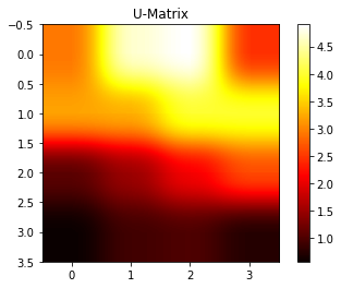
8 Forecasting
8.1 Fit an ARIMA model to a timeseries.
a) Plot the timeseries.
# Read in new data set
air = pd.read_csv('/Users/air.csv')

air["DATE"] = pd.to_datetime(air["DATE"], infer_datetime_format = True)
air.index = air["DATE"].values

plt.plot(air.index, air["AIR"])
plt.show()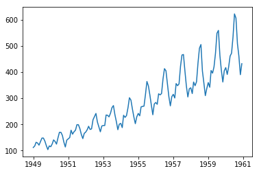
b) Fit an ARIMA model and predict 2 years (24 months).
import pyflux as pf

# ar = 12 is necessary to indicate the seasonality of data
model = pf.ARIMA(data = air, ar = 12, ma = 1, integ = 0, target = 'AIR',
                 family = pf.Normal())
x = model.fit("MLE")
model.plot_predict(h = 24)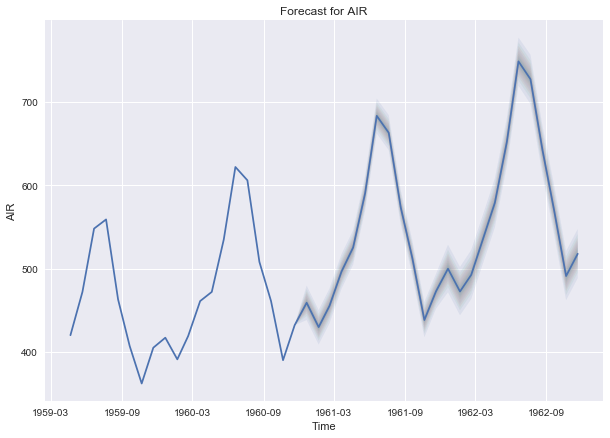
8.2 Fit a Simple Exponential Smoothing model to a timeseries.
a) Plot the timeseries.
# Read in new data set
usecon = pd.read_csv('/Users/usecon.csv')

petrol = usecon["PETROL"]

plt.plot(petrol)
plt.show()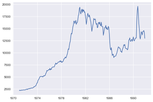
b) Fit a Simple Exponential Smoothing model, predict 2 years (24 months) out and plot predictions.
Currently, there is not a good package in Python to fit a simple exponential smoothing model. The formula for fitting an exponential smoothing model is not difficult, so we can do it by creating our own functions in Python.
The simplest form of exponential smoothing is given by, where \(t > 0\):
\[Eq1: s_0 = x_0\]
\[Eq2: s_t = \alpha x_t + (1 - \alpha)s_{t-1}\] Therefore, we can implement a simple exponential smoothing model as follows:
def simple_exp_smoothing(data, alpha, n_preds):
    # Eq1:
    output = [data[0]]
    # Smooth given data plus we want to predict 24 units
    # past the end
    for i in range(1, len(data) + n_preds):
        # Eq2:
        if (i < len(data)):
            output.append(alpha * data[i] + (1 - alpha) * data[i-1])
        else:
            output.append(alpha * output[i-1] + (1 - alpha) * output[i-2])
    return output

pred = simple_exp_smoothing(petrol, 0.9999, 24)

plt.plot(pd.DataFrame(pred), color = "red")
plt.plot(petrol, color = "blue")
plt.show()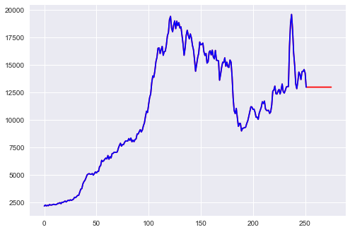
8.3 Fit a Holt-Winters model to a timeseries.
a) Plot the timeseries.
vehicle = usecon["VEHICLE"]

plt.plot(vehicle)
plt.show()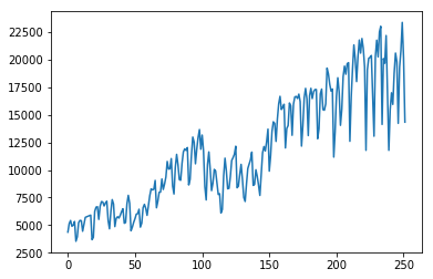
b) Fit a Holt-Winters additive model, predict 2 years (24 months) out and plot predictions.
Currently, there is not a good package in Python to fit a Holt-Winters additive model. The formula for fitting a Holt-Winters additive model is not difficult, so we can do it by creating our own functions in Python.
The following is an implementation of the Holt-Winters additive model given at triple exponential smoothing code.
def initial_trend(series, slen):
    sum = 0.0
    for i in range(slen):
        sum += float(series[i+slen] - series[i]) / slen
    return sum / slen
def initial_seasonal_components(series, slen):
    seasonals = {}
    season_averages = []
    n_seasons = int(len(series)/slen)
    # compute season averages
    for j in range(n_seasons):
        season_averages.append(sum(series[slen*j:slen*j+slen])/float(slen))
    # compute initial values
    for i in range(slen):
        sum_of_vals_over_avg = 0.0
        for j in range(n_seasons):
            sum_of_vals_over_avg += series[slen*j+i]-season_averages[j]
        seasonals[i] = sum_of_vals_over_avg/n_seasons
    return seasonals
def triple_exponential_smoothing_add(series, slen, alpha, beta, gamma,
                                     n_preds):
    result = []
    seasonals = initial_seasonal_components(series, slen)
    for i in range(len(series)+n_preds):
        if i == 0: # initial values
            smooth = series[0]
            trend = initial_trend(series, slen)
            result.append(series[0])
            continue
        if i >= len(series): # we are forecasting
            m = i - len(series) + 1
            result.append((smooth + m*trend) + seasonals[i%slen])
        else:
            val = series[i]
            last_smooth, smooth = smooth, alpha*(val-seasonals[i%slen])
                                                 + (1-alpha)*(smooth+trend)
            trend = beta * (smooth-last_smooth) + (1-beta)*trend
            seasonals[i%slen] = gamma*(val-smooth) +
                                (1-gamma)*seasonals[i%slen]
            result.append(smooth+trend+seasonals[i%slen])
    return result

add_preds = triple_exponential_smoothing_add(vehicles, 12, 0.5731265, 0,
                                             0.7230956, 24)

plt.plot(pd.DataFrame(add_preds), color = "red")
plt.plot(vehicles, color = "blue")
plt.show()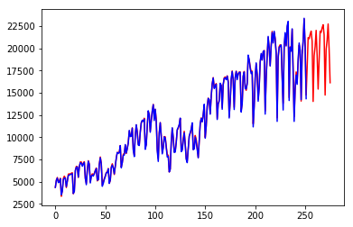
8.4 Fit a Facebook Prophet forecasting model to a timeseries.
from fbprophet import Prophet

air = pd.read_csv("/Users/air.csv")

air_df = pd.DataFrame()

air_df["ds"] = pd.to_datetime(air["DATE"], infer_datetime_format = True)
air_df["y"] = air["AIR"]

m = Prophet(yearly_seasonality = True, weekly_seasonality = False)

m.fit(air_df)

future = m.make_future_dataframe(periods = 24, freq = "M")

forecast = m.predict(future)

m.plot(forecast)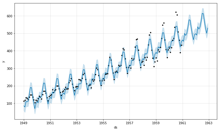
9 Model Evaluation & Selection
9.1 Evaluate the accuracy of regression models.
a) Evaluation on training data.
train = pd.read_csv('/Users/boston_train.csv')
test = pd.read_csv('/Users/boston_test.csv')

# Random Forest Regression Model
from sklearn.ensemble import RandomForestRegressor
rfMod = RandomForestRegressor(random_state=29)
rfMod.fit(train.drop(["Target"], axis = 1), train["Target"])

# Evaluation on training data
predY = rfMod.predict(train.drop(["Target"], axis = 1))

# Determine coefficient of determination score
from sklearn.metrics import r2_score
r2_rf = r2_score(train["Target"], predY)
print("Random forest regression model r^2 score (coefficient of determination): %f" % r2_rf)
## Random forest regression model r^2 score (coefficient of determination): 0.975233b) Evaluation on testing data.
# Random Forest Regression Model (rfMod)

# Evaluation on testing data
predY = rfMod.predict(test.drop(["Target"], axis = 1))

# Determine coefficient of determination score
r2_rf = r2_score(test["Target"], predY)
print("Random forest regression model r^2 score (coefficient of determination): %f" % r2_rf)
## Random forest regression model r^2 score (coefficient of determination): 0.833687The sklearn metric r2_score is only one option for assessing a regression model. Please go here for more information about other sklearn regression metrics.
9.2 Evaluate the accuracy of classification models.
a) Evaluation on training data.
train = pd.read_csv('/Users/digits_train.csv')
test = pd.read_csv('/Users/digits_test.csv')

# Random Forest Classification Model
from sklearn.ensemble import RandomForestClassifier
rfMod = RandomForestClassifier(random_state=29)
rfMod.fit(train.drop(["Target"], axis = 1), train["Target"])

# Evaluation on training data
predY = rfMod.predict(train.drop(["Target"], axis = 1))

# Determine accuracy score
from sklearn.metrics import accuracy_score
accuracy_rf = accuracy_score(train["Target"], predY)
print("Random forest model accuracy: %f" % accuracy_rf)
## Random forest model accuracy: 1.000000b) Evaluation on testing data.
# Random Forest Classification Model (rfMod)

# Evaluation on testing data
predY = rfMod.predict(test.drop(["Target"], axis = 1))

# Determine accuracy score
accuracy_rf = accuracy_score(test["Target"], predY)
print("Random forest model accuracy: %f" % accuracy_rf)
## Random forest model accuracy: 0.940741Note: The sklearn metric accuracy_score is only one option for assessing a classification model. Please go here for more information about other sklearn classification metrics.
Appendix
1 Built-in Python Data Types
Sequences
Sets
Mapping:
2 Python Plotting Packages
Bokeh
A Python package which is useful for interactive visualizations and is optimized for web browser presentations.
PyPlot
A Python package which is useful for data plotting and visualization.
Seaborn
A Python package which is useful for data plotting and visualization. In particular, Seaborn includes tools for drawing attractive statistical graphics.
3 Python packages used in this tutorial
pandas
Working with data structures and performing data analysis
NumPy
Scientific and mathematical computing
re
Regular expressions
Decimal
Tools for decimal floating point arithmetic
sklearn
scikit-learn, or more commonly known as sklearn, is useful for basic and advanced data mining, machine learning, and data analysis. sklearn includes tools for classification, regression, clustering, dimensionality reduction, model selection, and data pre-processing.
statsmodels.api
Tools for the estimation of many different statistical models
xgboost
Extreme gradient boosting models
pyclustering
Tools for clustering input data
PyFlux
Tools for time series analysis and prediction
Alphabetical Index
Array
A NumPy array is a data type in which the elements of the array are all of the same type. Please see the following example of array creation and access:
import numpy as np
my_array = np.array([1, 2, 3, 4])
print(my_array)
## [1 2 3 4]print(my_array[3])## 4Bytes & Byte arrays
A byte is a sequence of integers which is immutable, whereas a byte array is its mutable counterpart.
Data Frame
A two-dimensional tabular structure with labeled axes (rows and columns), where data observations are represented by rows and data variables are represented by columns.
Dictionary
An associative array which is indexed by keys which map to values. Therefore, a dictionary is an unordered set of key:value pairs where each key is unique. Please see the following example of dictionary creation and access:
import pandas as pd
student = pd.read_csv('/Users/class.csv')
for_dict = pd.concat([student["Name"], student["Age"]], axis = 1)
class_dict = for_dict.set_index('Name').T.to_dict('list')
print(class_dict.get('James'))
## [12]List
A sequence of comma-separated objects that need not be of the same type. Please see the following example of list creation and access:
list1 = ['item1', 102]
print(list1)
## ['item1', 102]print(list1[1])## 102Python also has what are known as “Tuples”, which are immutable lists created in the same way as lists, except with paranthesis instead of brackets.
Series
A one-dimensional data frame. Please see the following example of Series creation and access:
import pandas as pd
my_array = pd.Series([1, 3, 5, 9])
print(my_array)
## 0 1
## 1 3
## 2 5
## 3 9
## dtype: int64print(my_array[1])## 3Sets & Frozen Sets
A set is a unordered collection of immutable objects. The difference between a set and a frozen set is that the former is mutable, while the latter is immutable. Please see the following example of set and frozen set creation and access:
s = set(["1", "2", "3"])
# s is a set, which means you can add or delete elements from s
print(s)
## {'2', '1', '3'}s.add("4")
print(s)## {'1', '3', '4', '2'}fs = frozenset(["1", "2", "3"])
# fs is a frozenset, which means you cannot add or delete elements from fs
print(fs)## frozenset({'3', '1', '2'})str
A list of characters, though characters are not a type in Python, but rather a string of length 1. Strings are indexable like arrays. Please see the following example of String creation and access:
s = 'My first string!'
print(s)
## My first string!print(s[5])## rFor more information on Python packages and functions, along with helpful examples, please see Python.