SAS Tutorial
Welcome to the SAS tutorial version of Data Science Rosetta Stone. Before beginning this tutorial, please check to make sure you have SAS 14.2 installed (this is not required, but this was the release used to generate the following examples). SAS Enterprise Miner Workstation 14.2 was used to produce some of the following results.
You also may need to insure that your SAS environment is connected with an R environment so that the R code that SAS calls at the end of this tutorial from the IML Procedure runs successfully.
Note: In SAS,
*  This is a single line comment ;
/* This is a paragraph
   comment */
Now let’s get started!
1 Reading in Data and Basic Statistical Functions
1.1 Read in the data.
The IMPORT Procedure is useful for reading in SAS data sets of a variety of different types.
a) Read the data in as a .csv file.
proc import out = student
  datafile = 'C:/Users/class.csv'
  dbms = csv replace;
  getnames = yes;
run;
b) Read the data in as a .xls file.
proc import out = student_xls
  datafile = 'C:/Users/class.xls'
  dbms = xls replace;
  getnames = yes;
run;
c) Read the data in as a .json file.
There is more code involved in reading a .json file into SAS so that all the format is correct, however we will not at this time dive into the explanation for all this code, but please see the links below.
data student_json;
  INFILE 'C:/Users/class.json' LRECL  = 3456677  TRUNCOVER SCANOVER
    dsd
    dlm=",}";
  INPUT
    @'"Name":' Name : $12.
    @'"Sex":' Sex : $2.
    @'"Age":' Age :
    @'"Height":' Height :
    @'"Weight":' Weight :
    @@;
run;1.2 Find the dimensions of the data set.
The shape of a SAS data set is available by running the IMPORT Procedure and looking at the notes in the log file.
proc import out = student
  datafile = 'C:/Users/class.csv'
  dbms = csv replace;
  getnames = yes;
run;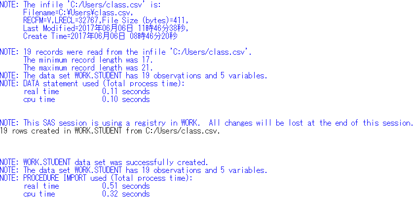
1.3 Find basic information about the data set.
The CONTENTS procedure prints information about a SAS data set.
proc contents data = student;
run;
The CONTENTS Procedure
Data Set Name WORK.STUDENT Observations 19
Member Type DATA Variables 5
Engine V9 Indexes 0
Created 07/05/2017 13:49:31 Observation Length 32
Last Modified 07/05/2017 13:49:31 Deleted Observations 0
Protection Compressed NO
Data Set Type Sorted NO
Label
Data Representation WINDOWS_64
Encoding wlatin1 Western (Windows)
Alphabetic List of Variables and Attributes
# Variable Type Len Format Informat
3 Age Num 8 BEST12. BEST32.
4 Height Num 8 BEST12. BEST32.
1 Name Char 7 $7. $7.
2 Sex Char 1 $1. $1.
5 Weight Num 8 BEST12. BEST32. 1.4 Look at the first 5 (last 5) observations.
The PRINT procedure prints a SAS data set, according to the specifications and options provided.
/* obs= option tells SAS how many observations to print, starting
   with the first observation */
proc print data = student (obs=5);
run;
Obs Name Sex Age Height Weight
1 Alfred M 14 69 112.5
2 Alice F 13 56.5 84
3 Barbara F 13 65.3 98
4 Carol F 14 62.8 102.5
5 Henry M 14 63.5 102.5–
/* print the last 5 observations */
proc print data = student (firstobs=15);
run;
Obs Name Sex Age Height Weight
15 Philip M 16 72 150
16 Robert M 12 64.8 128
17 Ronald M 15 67 133
18 Thomas M 11 57.5 85
19 William M 15 66.5 1121.5 Calculate means of numeric variables.
The MEANS procedure prints the means of all numeric variables of a SAS data set, as well as other descriptive statistics.
proc means data = student mean;
run;
The MEANS Procedure
Variable Mean
------------------------
Age 13.3157895
Height 62.3368421
Weight 100.0263158
------------------------1.6 Compute summary statistics of the data set.
Summary statistics of a SAS data set are available by running the MEANS procedure and specifying statistics to return.
/* SAS uses a different method than Python and R to compute
   quartiles, but the method in each language can be changed */
/* maxdec= option tells SAS to print at most 2 numbers behind
   the decimal point */
proc means data = student min q1 median mean q3 max n maxdec=2;
run;
The MEANS Procedure
Lower
Variable Minimum Quartile Median Mean
------------------------------------------------------------------------
Age 11.00 12.00 13.00 13.32
Height 51.30 57.50 62.80 62.34
Weight 50.50 84.00 99.50 100.03
------------------------------------------------------------------------
Upper
Variable Quartile Maximum N
----------------------------------------------
Age 15.00 16.00 19
Height 66.50 72.00 19
Weight 112.50 150.00 19
----------------------------------------------1.7 Descriptive statistics functions applied to columns of the data set.
/* The var statement tells SAS which variable to use for the
   procedure */
proc means data = student stddev sum n max min median maxdec=2;
  var Weight;
run;
The MEANS Procedure
Analysis Variable : Weight
Std Dev Sum N Maximum Minimum Median
------------------------------------------------------------------------
22.77 1900.50 19 150.00 50.50 99.50
------------------------------------------------------------------------1.8 Produce a one-way table to describe the frequency of a variable.
The FREQ procedure prints the frequency of categorical or discrete variables of a SAS data set.
a) Produce a one-way table of a discrete variable.
proc freq data = student;
  tables Age / nopercent norow nocol;
run;
The FREQ Procedure
Cumulative
Age Frequency Frequency
------------------------------
11 2 2
12 5 7
13 3 10
14 4 14
15 4 18
16 1 19 b) Produce a one-way table of a categorical variable.
proc freq data = student;
  tables Sex / nopercent norow nocol;
run;
The FREQ Procedure
Cumulative
Sex Frequency Frequency
------------------------------
F 9 9
M 10 19 The tables statement allows you to specify multiple variables at once, separated only by a space, so both of these tables could have been created with one FREQ procedure call. The options on the tables statement (nopercent norow nocol) prevent SAS from printing percents in the table, which are printed by default.
1.9 Produce a two-way table to visualize the frequency of two categorical (or discrete) variables.
/* The "*" between two variables on the tables statement
   indicates to produce a two-way table of the two variables */
proc freq data = student;
  tables Age*Sex / nopercent norow nocol;
run;
The FREQ Procedure
Table of Age by Sex
Age Sex
Frequency|F |M | Total
---------+--------+--------+
11 | 1 | 1 | 2
---------+--------+--------+
12 | 2 | 3 | 5
---------+--------+--------+
13 | 2 | 1 | 3
---------+--------+--------+
14 | 2 | 2 | 4
---------+--------+--------+
15 | 2 | 2 | 4
---------+--------+--------+
16 | 0 | 1 | 1
---------+--------+--------+
Total 9 10 191.10 Select a subset of the data that meets a certain criterion.
The SAS DATA step is used for all things data manipulation and in Section 2 we will explore it further.
data females;
  set student;
  where Sex = "F";
run;
proc print data = females(obs=5);
run;
Obs Name Sex Age Height Weight
1 Alice F 13 56.5 84
2 Barbara F 13 65.3 98
3 Carol F 14 62.8 102.5
4 Jane F 12 59.8 84.5
5 Janet F 15 62.5 112.51.11 Determine the correlation between two continuous variables.
/* The nosimple option reduces the output of this procedure */
proc corr data = student pearson nosimple;
var Height Weight;
run;
The CORR Procedure
2 Variables: Height Weight
Pearson Correlation Coefficients, N = 19
Prob > |r| under H0: Rho=0
Height Weight
Height 1.00000 0.87779
<.0001
Weight 0.87779 1.00000
<.0001 2 Basic Graphing and Plotting Functions
The SGPLOT procedure is a very useful SAS procedure for producing plots from data. For more information on other statements within the SGPLOT procedure, please see the Appendix Section 2.
2.1 Visualize a single continuous variable by producing a histogram.
proc sgplot data = student;
  histogram weight / binwidth=20 binstart=40 scale=count;
  xaxis values=(40 to 160 by 20);
run;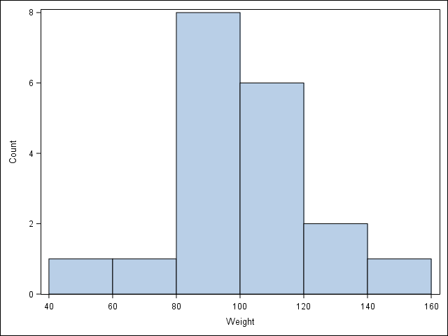
2.2 Visualize a single continuous variable by producing a boxplot.
/* SAS automatically prints the mean on the boxplot */
proc sgplot data = student;
  vbox Weight;
run;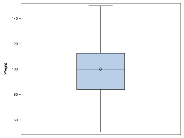
2.3 Visualize two continuous variables by producing a scatterplot.
/* Notice here you specify the y variable followed by the x variable */
proc sgscatter data = student;
  plot Weight * Height;
run; 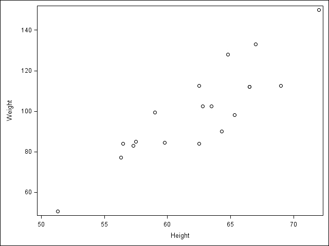
2.4 Visualize a relationship between two continuous variables by producing a scatterplot and a plotted line of best fit.
/* Use proc reg to get the parameter estimates for the line of best fit,
   but don't print the graph (ods graphics off) */
ods graphics off;
proc reg data = student;
  /* Syntax indicates Weight as a function of Height */
  model Weight = Height;
  ods output ParameterEstimates=PE;
run;
ods graphics on;

/* data _null_ indicates to not create a data set, but
   run the code within the data step to create macro
   variables to store the parameter estimates */
data _null_;
  set PE;
  if _n_=1 then call symput('Int', put(estimate, BEST6.));
  else call symput('Slope', put(estimate, BEST6.));
run;

/* Use proc sgplot with the reg statement so it prints the line of best fit,
   and use the inset statement to print the equation of the line
   of best fit */
proc sgplot data = student noautolegend;
  reg y = Weight x = Height;
  inset "Line: Y = &Slope x + &Int" / position=topleft;
run; 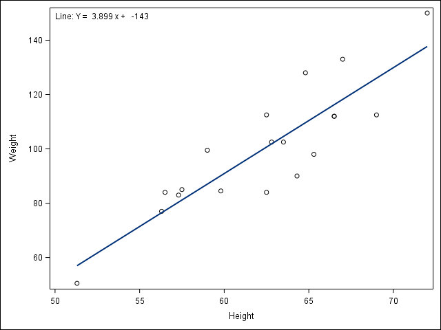
REG Procedure | set statement | macro variables | call symput()
2.5 Visualize a categorical variable by producing a bar chart.
/* Notice here you must first sort by Sex and then plot the vertical
  bar chart */
proc sort data = student;
  by Sex;
run;
proc sgplot data = student;
  vbar Sex;
run; 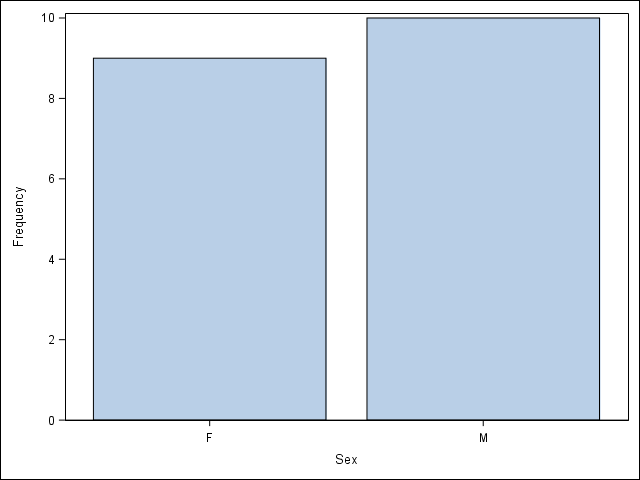
2.6 Visualize a continuous variable, grouped by a categorical variable, using side-by-side boxplots.
More advanced side-by-side boxplot with color.
proc sgplot data = student;
  vbox Weight / group=Sex;
run; 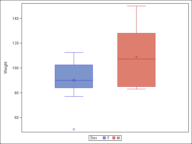
3 Basic Data Wrangling and Manipulation
Many of the following examples make use of the SAS DATA step for manipulating and altering data sets, and a main part of the DATA step is the set statement.
3.1 Create a new variable in a data set as a function of existing variables in the data set.
data student;
  set student;
  BMI = Weight / (Height**2) * 703;
run;
proc print data = student(obs=5);
run;
Obs Name Sex Age Height Weight BMI
1 Alfred M 14 69 112.5 16.6115
2 Alice F 13 56.5 84 18.4986
3 Barbara F 13 65.3 98 16.1568
4 Carol F 14 62.8 102.5 18.2709
5 Henry M 14 63.5 102.5 17.87033.2 Create a new variable in a data set using if/else logic of existing variables in the data set.
data student;
  set student;
  if (BMI < 19.0) then BMI_class = "Underweight";
  else BMI_class = "Healthy";
run;
proc print data = student(obs=5);
run;
Obs Name Sex Age Height Weight BMI BMI_class
1 Alfred M 14 69 112.5 16.6115 Underweight
2 Alice F 13 56.5 84 18.4986 Underweight
3 Barbara F 13 65.3 98 16.1568 Underweight
4 Carol F 14 62.8 102.5 18.2709 Underweight
5 Henry M 14 63.5 102.5 17.8703 Underweightif-then/else statement
3.3 Create a new variable in a data set using mathemtical functions applied to existing variables in the data set.
Using the log(), exp(), sqrt(), & abs() functions.
data student;
set student;
LogWeight = log(Weight);
ExpAge = exp(Age);
SqrtHeight = sqrt(Height);
if (BMI < 19.0) then BMI_Neg = -BMI;
else BMI_Neg = BMI;
BMI_Pos = abs(BMI_Neg);
/* Create a Boolean variable, which is handled differently
in SAS than in Python and R */
BMI_Check = (BMI_Pos = BMI);
run;
proc print data = student(obs=5);
run;
Obs Name    Sex          Age       Height       Weight   BMI    BMI_class

  1 Alfred   M            14           69        112.5 16.6115 Underweight
  2 Alice    F            13         56.5           84 18.4986 Underweight
  3 Barbara  F            13         65.3           98 16.1568 Underweight
  4 Carol    F            14         62.8        102.5 18.2709 Underweight
  5 Henry    M            14         63.5        102.5 17.8703 Underweight
Log Sqrt BMI_
Obs Weight ExpAge Height BMI_Neg BMI_Pos Check
1 4.72295 1202604.28 8.30662 -16.6115 16.6115 1
2 4.43082 442413.39 7.51665 -18.4986 18.4986 1
3 4.58497 442413.39 8.08084 -16.1568 16.1568 1
4 4.62986 1202604.28 7.92465 -18.2709 18.2709 1
5 4.62986 1202604.28 7.96869 -17.8703 17.8703 1 if-then/else statement
3.4 Drop variables from a data set.
data student;
  set student (drop = LogWeight ExpAge SqrtHeight BMI_Neg BMI_Pos BMI_Check);
run;
proc print data = student(obs=5);
run;
Obs Name Sex Age Height Weight BMI BMI_class
1 Alfred M 14 69 112.5 16.6115 Underweight
2 Alice F 13 56.5 84 18.4986 Underweight
3 Barbara F 13 65.3 98 16.1568 Underweight
4 Carol F 14 62.8 102.5 18.2709 Underweight
5 Henry M 14 63.5 102.5 17.8703 Underweightdrop= data set option
3.5 Sort a data set by a variable.
a) Sort data set by a continuous variable.
proc sort data = student;
  by Age;
run;
proc print data = student(obs=5);
run;
Obs Name Sex Age Height Weight BMI BMI_class
1 Joyce F 11 51.3 50.5 13.4900 Underweight
2 Thomas M 11 57.5 85 18.0733 Underweight
3 James M 12 57.3 83 17.7715 Underweight
4 Jane F 12 59.8 84.5 16.6115 Underweight
5 John M 12 59 99.5 20.0944 Healthy b) Sort data set by a categorical variable.
proc sort data = student;
  by Sex;
run;
/* Notice that the data is now sorted first by Sex and
   then within Sex by Age */
proc print data = student(obs=5);
run;
Obs Name Sex Age Height Weight BMI BMI_class
1 Joyce F 11 51.3 50.5 13.4900 Underweight
2 Jane F 12 59.8 84.5 16.6115 Underweight
3 Louise F 12 56.3 77 17.0777 Underweight
4 Alice F 13 56.5 84 18.4986 Underweight
5 Barbara F 13 65.3 98 16.1568 Underweight3.6 Compute descriptive statistics of continuous variables, grouped by a categorical variable.
proc means data = student mean;
  by Sex;
  var Age Height Weight BMI;
run;
---------------------------------- Sex=F ----------------------------------
The MEANS Procedure
Variable Mean
------------------------
Age 13.2222222
Height 60.5888889
Weight 90.1111111
BMI 17.0510391
------------------------
---------------------------------- Sex=M ----------------------------------
Variable Mean
------------------------
Age 13.4000000
Height 63.9100000
Weight 108.9500000
BMI 18.5942434
------------------------3.7 Add a new row to the bottom of a data set.
/* Look at the tail of the data currently */
proc print data = student(firstobs=15);
run;
Obs Name Sex Age Height Weight BMI BMI_class
15 Alfred M 14 69 112.5 16.6115 Underweight
16 Henry M 14 63.5 102.5 17.8703 Underweight
17 Ronald M 15 67 133 20.8285 Healthy
18 William M 15 66.5 112 17.8045 Underweight
19 Philip M 16 72 150 20.3414 Healthy data student;
set student end = eof;
output;
if eof then do;
Name = 'Jane';
Sex = 'F';
Age = 14;
Height = 56.3;
Weight = 77.0;
BMI = 17.077695;
BMI_Class = 'Underweight';
output;
end;
run;
proc print data = student(firstobs=16);
run;Obs Name Sex Age Height Weight BMI BMI_class
16 Henry M 14 63.5 102.5 17.8703 Underweight
17 Ronald M 15 67 133 20.8285 Healthy
18 William M 15 66.5 112 17.8045 Underweight
19 Philip M 16 72 150 20.3414 Healthy
20 Jane F 14 56.3 77 17.0777 Underweightif-then/else & output statements | do loop, end= & firstobs= data set options
3.8 Create a user-defined function and apply it to a variable in the data set to create a new variable in the data set.
proc fcmp outlib=sasuser.userfuncs.myfunc;
  function toKG(lb);
    kg = 0.45359237 * lb;
  return(kg);
endsub;

options cmplib=sasuser.userfuncs;

data studentKG;
  set student;
  Weight_KG = toKG(Weight);
run;

proc print data = studentKG(obs=5);
run;
   Obs    Name       Sex             Age          Height          Weight

     1    Joyce       F               11            51.3            50.5
     2    Jane        F               12            59.8            84.5
     3    Louise      F               12            56.3              77
     4    Alice       F               13            56.5              84
     5    Barbara     F               13            65.3              98

                                    Weight_
   Obs      BMI       BMI_class        KG

     1    13.4900    Underweight    22.9064
     2    16.6115    Underweight    38.3286
     3    17.0777    Underweight    34.9266
     4    18.4986    Underweight    38.1018
5 16.1568 Underweight 44.45214 More Advanced Data Wrangling
4.1 Drop observations with missing information.
/* Notice the use of the fish data set because it has some missing
   observations */
proc import out = fish
  datafile ='C:/Users/fish.csv'
  dbms = csv replace;
  getnames = yes;
run;

/* First sort by Weight, requesting those with NA for Weight first,
   which SAS does automatically */
proc sort data = fish;
  by Weight;
run;
proc print data = fish(obs=5);
run;
Obs Species Weight Length1 Length2
1 Bream . 29.5 32
2 Roach 0 19 20.5
3 Perch 5.9 7.5 8.4
4 Smelt 6.7 9.3 9.8
5 Smelt 7 10.1 10.6
Obs Length3 Height Width
1 37.3 13.9129 5.0728
2 22.8 6.4752 3.3516
3 8.8 2.112 1.408
4 10.8 1.7388 1.0476
5 11.6 1.7284 1.1484data new_fish;
set fish;
/* Notice the not-equal operator (^=) and how SAS denotes
missing values (.) */
if (Weight ^= .);
run;
proc print data = new_fish(obs=5);
run; Obs Species Weight Length1 Length2
1 Roach 0 19 20.5
2 Perch 5.9 7.5 8.4
3 Smelt 6.7 9.3 9.8
4 Smelt 7 10.1 10.6
5 Smelt 7.5 10 10.5
Obs Length3 Height Width
1 22.8 6.4752 3.3516
2 8.8 2.112 1.408
3 10.8 1.7388 1.0476
4 11.6 1.7284 1.1484
5 11.6 1.972 1.16SORT Procedure | if-then/else statement
4.2 Merge two data sets together on a common variable.
a) First, select specific columns of a data set to create two smaller data sets.
/* Notice the use of the student data set again, however we want to reload it
   without the changes we've made previously  */
proc import out = student
  datafile = 'C:/Users/class.csv'
  dbms = csv replace;
  getnames = yes;
run;
data student1;
  set student(keep= Name Sex Age);
run;
proc print data = student1(obs=5);
run;
Obs Name Sex Age
1 Alfred M 14
2 Alice F 13
3 Barbara F 13
4 Carol F 14
5 Henry M 14data student2;
set student(keep= Name Height Weight);
run;
proc print data = student2(obs=5);
run; Obs Name Height Weight
1 Alfred 69 112.5
2 Alice 56.5 84
3 Barbara 65.3 98
4 Carol 62.8 102.5
5 Henry 63.5 102.5keep= data set option
b) Second, we want to merge the two smaller data sets on the common variable.
data new;
  merge student1 student2;
  by Name;
run;
proc print data = new(obs=5);
run;
Obs Name Sex Age Height Weight
1 Alfred M 14 69 112.5
2 Alice F 13 56.5 84
3 Barbara F 13 65.3 98
4 Carol F 14 62.8 102.5
5 Henry M 14 63.5 102.5c) Finally, we want to check to see if the merged data set is the same as the original data set.
proc compare base = student compare = new brief;
run;
The COMPARE Procedure
Comparison of WORK.STUDENT with WORK.NEW
(Method=EXACT)
NOTE: No unequal values were found. All values compared are exactly equal.4.3 Merge two data sets together by index number only.
a) First, select specific columns of a data set to create two smaller data sets.
data newstudent1;
  set student(keep= Name Sex Age);
run;
proc print data = newstudent1(obs=5);
run;
Obs Name Sex Age
1 Alfred M 14
2 Alice F 13
3 Barbara F 13
4 Carol F 14
5 Henry M 14data newstudent2;
set student(keep= Height Weight);
run;
proc print data = newstudent2(obs=5);
run; Obs Height Weight
1 69 112.5
2 56.5 84
3 65.3 98
4 62.8 102.5
5 63.5 102.5keep= data set option
b) Second, we want to join the two smaller data sets.
data new2;
  merge newstudent1 newstudent2;
run;
proc print data = new2(obs=5);
run;
Obs Name Sex Age Height Weight
1 Alfred M 14 69 112.5
2 Alice F 13 56.5 84
3 Barbara F 13 65.3 98
4 Carol F 14 62.8 102.5
5 Henry M 14 63.5 102.5merge statement
c) Finally, we want to check to see if the joined data set is the same as the original data set.
proc compare base = student compare = new2 brief;
run;
The COMPARE Procedure
Comparison of WORK.STUDENT with WORK.NEW2
(Method=EXACT)
NOTE: No unequal values were found. All values compared are exactly equal.4.4 Create a pivot table to summarize information about a data set.
/* Notice we are using a new data set that needs to be read into the
   environment */
proc import out = price
  datafile = 'C:/Users/price.csv'
  dbms = csv replace;
  getnames = yes;
run;

/* The following code is used to remove the "," and "$" characters from the
   ACTUAL column so that values can be summed */
data price;
  set price;
  num_actual = input(actual, dollar10.);
run;

proc sql;
  create table categorysales as
    select country, state, prodtype,
    product, sum(num_actual) as REVENUE
    from price
  group by country, state, prodtype, product;
quit;
proc print data = categorysales(obs=5);
run;
Obs COUNTRY STATE PRODTYPE PRODUCT REVENUE
1 Canada British Co FURNITURE BED 197706.6
2 Canada British Co FURNITURE SOFA 216282.6
3 Canada British Co OFFICE CHAI 200905.2
4 Canada British Co OFFICE DESK 186262.2
5 Canada Ontario FURNITURE BED 194493.6input() function | SQL Procedure
4.5 Return all unique values from a text variable.
proc iml;
  use price;
    read all var {STATE};
  close price;

  unique_states = unique(STATE);
  print(unique_states);
quit;
unique_states
COL1 COL2 COL3 COL4 COL5 COL6
ROW1 Baja Calif British Co California Campeche Colorado Florida
unique_states
COL7 COL8 COL9 COL10 COL11 COL12
ROW1 Illinois Michoacan New York North Caro Nuevo Leon Ontario
unique_states
COL13 COL14 COL15 COL16
ROW1 Quebec Saskatchew Texas WashingtonIML Procedure | unique() function
5 Preparation & Basic Regression
5.1 Pre-process a data set using principal component analysis.
/* Notice we are using a new data set that needs to be read into the
   environment */
proc import out = iris
  datafile = 'C:/Users/iris.csv'
  dbms = csv replace;
  getnames = yes;
run;

data features;
  set iris(drop=Target);
run;

proc princomp data = features noprint outstat = feat_princomp;
  var SepalLength SepalWidth PetalLength PetalWidth;
run;

data eigenvectors;
    set feat_princomp;
    where _TYPE_ = "SCORE";
run;
proc print data = eigenvectors;
run;
Sepal Sepal Petal Petal
Obs _TYPE_ _NAME_ Length Width Length Width
1 SCORE Prin1 0.52237 -0.26335 0.58125 0.56561
2 SCORE Prin2 0.37232 0.92556 0.02109 0.06542
3 SCORE Prin3 -0.72102 0.24203 0.14089 0.63380
4 SCORE Prin4 -0.26200 0.12413 0.80115 -0.52355drop= data set option | PRINCOMP Procedure
5.2 Split data into training and testing data and export as a .csv file.
/* outall option tells SAS to add a flag showing which observations were
   chosen */
/* seed = 29 specifies the seed for random values so the results are
   reproducible */
proc surveyselect data = iris outall out = all method = srs samprate = 0.7
                              seed = 29;
run;

data train (drop = selected) test (drop = selected);
    set all;
    if (selected = 1) then output train;
  else output test;
run;

proc export data = train
   outfile = 'C:\Users\iris_train.csv'
   dbms = csv;
run;
proc export data = test
   outfile = 'C:\Users\iris_test.csv'
   dbms = csv;
run;
SURVEYSELECT Procedure | drop= data set option | EXPORT Procedure
5.3 Fit a logistic regression model.
/* Notice we are using a new data set that needs to be read into the
   environment */
proc import out = tips
  datafile = 'C:/Users/tips.csv'
  dbms = csv replace;
  getnames = yes;
run;

/* The following code is used to determine if the individual left more than
   a 15% tip */
data tips;
  set tips;
  if (tip > 0.15*total_bill) then greater15 = 1;
  else greater15 = 0;
run;

/* The descending option tells SAS to model the probability that
  greater15 = 1 */
proc genmod data=tips descending;
  model greater15 = total_bill / dist = bin link = logit lrci;
run;
The GENMOD Procedure
Model Information
Data Set WORK.TIPS
Distribution Binomial
Link Function Logit
Dependent Variable greater15
Number of Observations Read 244
Number of Observations Used 244
Number of Events 135
Number of Trials 244
Response Profile
Ordered Total
Value greater15 Frequency
1 1 135
2 0 109
proc genmod is modeling the probability that greater15='1'.
Criteria For Assessing Goodness Of Fit
Criterion DF Value Value/DF
Log Likelihood -156.8714
Full Log Likelihood -156.8714
AIC (smaller is better) 317.7428
AICC (smaller is better) 317.7926
BIC (smaller is better) 324.7371
Algorithm converged.
Analysis Of Maximum Likelihood Parameter Estimates
Likelihood Ratio
Standard 95% Confidence Wald
Parameter DF Estimate Error Limits Chi-Square
Intercept 1 1.6477 0.3547 0.9722 2.3667 21.58
total_bill 1 -0.0725 0.0168 -0.1069 -0.0408 18.65
Scale 0 1.0000 0.0000 1.0000 1.0000
Analysis Of Maximum
Likelihood Parameter
Estimates
Parameter Pr > ChiSq
Intercept <.0001
total_bill <.0001
Scale
NOTE: The scale parameter was held fixed.if-then/else statement | GENMOD Procedure
5.4 Fit a linear regression model.
/* Fit a linear regression model of tip by total_bill */
proc reg data = tips outest=RegOut;
    tip_hat: model tip = total_bill;
quit;
The REG Procedure
Model: tip_hat
Dependent Variable: tip
Number of Observations Read 244
Number of Observations Used 244
Analysis of Variance
Sum of Mean
Source DF Squares Square F Value Pr > F
Model 1 212.42373 212.42373 203.36 <.0001
Error 242 252.78874 1.04458
Corrected Total 243 465.21248
Root MSE 1.02205 R-Square 0.4566
Dependent Mean 2.99828 Adj R-Sq 0.4544
Coeff Var 34.08782
Parameter Estimates
Parameter Standard
Variable DF Estimate Error t Value Pr > |t|
Intercept 1 0.92027 0.15973 5.76 <.0001
total_bill 1 0.10502 0.00736 14.26 <.00016 Supervised Machine Learning
6.1 Fit a logistic regression model on training data and assess against testing data.
a) Fit a logistic regression model on training data.
/* Notice we are using new data sets that need to be read into the
   environment */
proc import out = train
  datafile = 'C:/Users/tips_train.csv'
  dbms = csv replace;
  getnames = yes;
run;
proc import out = test
  datafile = 'C:/Users/tips_test.csv'
  dbms = csv replace;
  getnames = yes;
run;

/* The following code is used to determine if the individual left more than
   a 15% tip */
data train;
  set train;
  if (tip > 0.15*total_bill) then greater15 = 1;
  else greater15 = 0;
run;
data test;
  set test;
  if (tip > 0.15*total_bill) then greater15 = 1;
  else greater15 = 0;
run;

/* The descending option tells SAS to model the probability that
  greater15 = 1 */
proc genmod data=train descending;
  model greater15 = total_bill / dist = bin link = logit lrci;
  store out = logmod;
run;
The GENMOD Procedure
Model Information
Data Set WORK.TRAIN
Distribution Binomial
Link Function Logit
Dependent Variable greater15
Number of Observations Read 195
Number of Observations Used 195
Number of Events 109
Number of Trials 195
Response Profile
Ordered Total
Value greater15 Frequency
1 1 109
2 0 86
proc genmod is modeling the probability that greater15='1'.
Criteria For Assessing Goodness Of Fit
Criterion DF Value Value/DF
Log Likelihood -125.2918
Full Log Likelihood -125.2918
AIC (smaller is better) 254.5836
AICC (smaller is better) 254.6461
BIC (smaller is better) 261.1296
Algorithm converged.
Analysis Of Maximum Likelihood Parameter Estimates
Likelihood Ratio
Standard 95% Confidence Wald
Parameter DF Estimate Error Limits Chi-Square
Intercept 1 1.6461 0.3946 0.8973 2.4501 17.40
total_bill 1 -0.0706 0.0185 -0.1088 -0.0359 14.59
Scale 0 1.0000 0.0000 1.0000 1.0000
Analysis Of Maximum
Likelihood Parameter
Estimates
Parameter Pr > ChiSq
Intercept <.0001
total_bill 0.0001
Scale
NOTE: The scale parameter was held fixed.b) Assess the model against the testing data.
/* Prediction on testing data */
proc plm source = logmod noprint;
    score data = test out = preds pred = pred / ilink;
run;

/* Determine how many were correctly classified */
data preds;
    set preds;
    if (pred < 0.5) then label = 0;
    else label = 1;
    if (label = greater15) then Result = "Correct";
    else Result = "Wrong";
run;

proc freq data = preds;
tables Result / nopercent norow nocol;
run;
The FREQ Procedure
Cumulative
Result Frequency Frequency
----------------------------------
Correct 34 34
Wrong 15 49 6.2 Fit a linear regression model on training data and assess against testing data.
a) Fit a linear regression model on training data.
/* Notice we are using new data sets that need to be read into the
  environment */
proc import out = train
  datafile = 'C:/Users/boston_train.csv'
  dbms = csv replace;
  getnames = yes;
run;
proc import out = test
  datafile = 'C:/Users/boston_test.csv'
  dbms = csv replace;
  getnames = yes;
run;

proc reg data = train outest=RegOut;
  predY: model Target = _0-_12;
quit;
The REG Procedure
Model: predY
Dependent Variable: Target
Number of Observations Read 354
Number of Observations Used 354
Analysis of Variance
Sum of Mean
Source DF Squares Square F Value Pr > F
Model 13 22145 1703.47137 68.48 <.0001
Error 340 8458.20364 24.87707
Corrected Total 353 30603
Root MSE 4.98769 R-Square 0.7236
Dependent Mean 22.48249 Adj R-Sq 0.7131
Coeff Var 22.18479
Parameter Estimates
Parameter Standard
Variable DF Estimate Error t Value Pr > |t|
Intercept 1 36.10820 6.50497 5.55 <.0001
_0 1 -0.08563 0.04277 -2.00 0.0461
_1 1 0.04603 0.01715 2.68 0.0076
_2 1 0.03641 0.07601 0.48 0.6322
_3 1 3.24796 1.07414 3.02 0.0027
_4 1 -14.87294 4.63609 -3.21 0.0015
_5 1 3.57687 0.53699 6.66 <.0001
_6 1 -0.00870 0.01685 -0.52 0.6059
_7 1 -1.36890 0.25296 -5.41 <.0001
_8 1 0.31312 0.08237 3.80 0.0002
_9 1 -0.01288 0.00460 -2.80 0.0054
_10 1 -0.97690 0.17100 -5.71 <.0001
_11 1 0.01133 0.00336 3.37 0.0008
_12 1 -0.52672 0.06256 -8.42 <.0001b) Assess the model against the testing data.
/* Predicton on testing data */
proc score data = test score=RegOut type=parms predict out = Pred;
    var _0-_12;
run;

/* Compute the squared differences between predicted and target */
data Pred;
    set Pred;
    sq_error = (predY - Target)**2;
run;

/* Compute the mean of the squared differences (mean squared error) as an
   assessment of the model */
proc means data = Pred mean;
  var sq_error;
run;
The MEANS Procedure
Analysis Variable : sq_error
Mean
------------
17.7713080
------------6.3 Fit a decision tree model on training data and assess against testing data.
a) Fit a decision tree classification model.
i) Fit a decision tree classification model on training data and determine variable importance
/* Notice we are using new data sets that need to be read into the
   environment */
proc import out = train
    datafile = 'C:/Users/breastcancer_train.csv'
    dbms = csv replace;
    getnames = yes;
run;
proc import out = test
    datafile = 'C:/Users/breastcancer_test.csv'
    dbms = csv replace;
    getnames = yes;
run;

/* HPSPLIT procedure is used to fit a decision tree model */
proc hpsplit data = train seed = 29;
    target Target;
    input _0-_29;
    /* Export information about variable importance */
    output importance=import;
    /* Export the model code so this can be used to score testing data */
    code file='hpbreastcancer.sas';
run;

/* Output of this model gives assessment against training data
     and variable importance */
The HPSPLIT Procedure
Performance Information
Execution Mode Single-Machine
Number of Threads 4
Data Access Information
Data Engine Role Path
WORK.TRAIN V9 Input On Client
Model Information
Split Criterion Used Entropy
Pruning Method Cost-Complexity
Subtree Evaluation Criterion Cost-Complexity
Number of Branches 2
Maximum Tree Depth Requested 10
Maximum Tree Depth Achieved 6
Tree Depth 3
Number of Leaves Before Pruning 15
Number of Leaves After Pruning 6
Model Event Level 1
Number of Observations Read 398
Number of Observations Used 398
The HPSPLIT Procedure
Model-Based Confusion Matrix
Predicted Error
Actual 1 0 Rate
1 242 1 0.0041
0 10 145 0.0645
Model-Based Fit Statistics for Selected Tree
N Mis-
Leaves ASE class Sensitivity Specificity Entropy Gini RSS
6 0.0229 0.0276 0.9959 0.9355 0.1297 0.0457 18.2063
Model-Based Fit Statistics for Selected Tree
AUC
0.9852
Variable Importance
Training
Variable Relative Importance Count
_23 1.0000 11.2865 1
_27 0.4072 4.5962 1
_1 0.3487 3.9356 2
_6 0.2355 2.6581 1ii. Assess the model against the testing data.
/* Score the test data using the model code */
data scored;
    set test;
    %include 'hpbreastcancer.sas';
run;

/* Use prediction probabilities to generate predictions, and compare these
     to the true responses */
/* If the prediction probability is less than 0.5, classify this as a 0
   and otherwise classify as a 1.  This isn't the best method -- a better
   method would be randomly assigning a 0 or 1 when a probability of 0.5
   occurrs, but this insures that results are consistent */
data scored;
    set scored;
    if (P_Target1 < 0.5) then prediction = 0;
    else prediction = 1;
    if (Target = prediction) then Result = "Correct";
  else Result = "Wrong";
run;

/* Determine how many were correctly classified */
proc freq data = scored;
  tables Result / nopercent norow nocol;
run;
The FREQ Procedure
Cumulative
Result Frequency Frequency
----------------------------------
Correct 157 157
Wrong 14 171 HPSPLIT Procedure | %include & if-then/else statements | FREQ Procedure
b) Fit a decision tree regression model.
i) Fit a decision tree regression model on training data and determine variable importance.
proc import out = train
    datafile = 'C:/Users/boston_train.csv'
    dbms = csv replace;
    getnames = yes;
run;
proc import out = test
    datafile = 'C:/Users/boston_test.csv'
    dbms = csv replace;
    getnames = yes;
run;

/* HPSPLIT procedure is used to fit a decision tree model */
proc hpsplit data = train seed = 29;
    target Target / level = int;
    input _0-_12;
    /* Export information about variable importance */
    output importance=import;
    /* Export the model code so this can be used to score testing data */
    code file='hpboston.sas';
run;

/* Output of this model gives assessment against training data
   and variable importance */
The HPSPLIT Procedure
Performance Information
Execution Mode Single-Machine
Number of Threads 4
Data Access Information
Data Engine Role Path
WORK.TRAIN V9 Input On Client
Model Information
Split Criterion Used Variance
Pruning Method Cost-Complexity
Subtree Evaluation Criterion Cost-Complexity
Number of Branches 2
Maximum Tree Depth Requested 10
Maximum Tree Depth Achieved 10
Tree Depth 10
Number of Leaves Before Pruning 188
Number of Leaves After Pruning 101
Number of Observations Read 354
Number of Observations Used 354
The HPSPLIT Procedure
Model-Based Fit Statistics for Selected Tree
N
Leaves ASE RSS
101 0.9750 345.2
Variable Importance
Training
Variable Relative Importance Count
_5 1.0000 132.8 13
_12 0.6026 79.9998 16
_7 0.3968 52.6772 9
_4 0.2663 35.3541 12
_0 0.2324 30.8579 7
_9 0.1574 20.8933 8
_6 0.1202 15.9544 12
_10 0.1063 14.1112 4
_11 0.0855 11.3541 8
_2 0.0713 9.4695 5
_8 0.0696 9.2408 3
_1 0.0583 7.7437 3ii. Assess the model against the testing data.
/* Score the test data using the model code */
data scored;
    set test;
    %include 'hpboston.sas';
run;

/* Compute the squared differences between predicted and target */
data scored;
    set scored;
    sq_error = (P_Target - Target)**2;
run;

/* Compute the mean of the squared differences (mean squared error) as an
     assessment of the model */
proc means data = scored mean;
  var sq_error;
run;
The MEANS Procedure
Analysis Variable : sq_error
Mean
------------
24.6222895
------------HPSPLIT Procedure | %include statement | MEANS Procedure
6.4 Fit a random forest model on training data and assess against testing data.
a) Fit a random forest classification model.
i) Fit a random forest classification model on training data and determine variable importance.
proc import out = train
    datafile = 'C:/Users/breastcancer_train.csv'
    dbms = csv replace;
    getnames = yes;
run;
proc import out = test
    datafile = 'C:/Users/breastcancer_test.csv'
    dbms = csv replace;
    getnames = yes;
run;

/* Output includes information about variable importance */
proc hpforest data = train;
    input _0 - _29 / level = interval;
    target Target / level = nominal;
    save file = 'hpbreastcancer2.bin';
run;
The HPFOREST Procedure
Performance Information
Execution Mode Single-Machine
Number of Threads 4
Data Access Information
Data Engine Role Path
WORK.TRAIN V9 Input On Client
Model Information
Parameter Value
Variables to Try 5 (Default)
Maximum Trees 100 (Default)
Inbag Fraction 0.6 (Default)
Prune Fraction 0 (Default)
Prune Threshold 0.1 (Default)
Leaf Fraction 0.00001 (Default)
Leaf Size Setting 1 (Default)
Leaf Size Used 1
Category Bins 30 (Default)
Interval Bins 100
Minimum Category Size 5 (Default)
Node Size 100000 (Default)
Maximum Depth 20 (Default)
Alpha 1 (Default)
Exhaustive 5000 (Default)
Rows of Sequence to Skip 5 (Default)
Split Criterion . Gini
Preselection Method . BinnedSearch
Missing Value Handling . Valid value
Number of Observations
Type N
Number of Observations Read 398
Number of Observations Used 398
Baseline Fit Statistics
Statistic Value
Average Square Error 0.238
Misclassification Rate 0.389
Log Loss 0.669
Fit Statistics
Average Average
Square Square Misclassification
Number Number Error Error Rate
of Trees of Leaves (Train) (OOB) (Train)
1 16 0.03015 0.0750 0.03015
2 35 0.01947 0.0739 0.04523
3 53 0.01284 0.0724 0.00754
4 66 0.01225 0.0658 0.01005
5 80 0.01156 0.0700 0.00754
6 92 0.01124 0.0712 0.00754
7 106 0.00938 0.0633 0.00251
8 122 0.00879 0.0623 0.00000
9 139 0.00887 0.0611 0.00000
10 157 0.00867 0.0611 0.00000
11 171 0.00889 0.0589 0.00251
12 188 0.00874 0.0557 0.00000
13 203 0.00847 0.0551 0.00000
14 223 0.00841 0.0552 0.00000
15 241 0.00804 0.0537 0.00251
16 253 0.00795 0.0496 0.00251
17 268 0.00827 0.0489 0.00503
18 283 0.00813 0.0485 0.00251
19 300 0.00793 0.0471 0.00251
20 315 0.00783 0.0471 0.00251
21 329 0.00763 0.0465 0.00251
22 345 0.00747 0.0453 0.00000
23 361 0.00740 0.0448 0.00000
24 375 0.00744 0.0442 0.00000
25 392 0.00749 0.0449 0.00251
26 406 0.00764 0.0448 0.00251
27 420 0.00750 0.0440 0.00251
28 437 0.00764 0.0438 0.00000
29 451 0.00776 0.0431 0.00000
30 466 0.00774 0.0426 0.00000
31 484 0.00778 0.0432 0.00251
32 502 0.00759 0.0426 0.00000
33 518 0.00749 0.0420 0.00251
34 535 0.00747 0.0418 0.00000
35 550 0.00742 0.0415 0.00000
36 562 0.00746 0.0411 0.00000
37 578 0.00741 0.0411 0.00000
38 594 0.00731 0.0404 0.00000
39 609 0.00717 0.0407 0.00000
40 623 0.00720 0.0404 0.00000
41 642 0.00712 0.0405 0.00000
42 661 0.00702 0.0399 0.00000
43 679 0.00687 0.0397 0.00000
44 692 0.00677 0.0396 0.00000
45 710 0.00665 0.0392 0.00000
46 731 0.00652 0.0391 0.00000
47 741 0.00654 0.0387 0.00000
48 754 0.00661 0.0392 0.00000
49 769 0.00656 0.0393 0.00000
50 780 0.00657 0.0395 0.00000
51 795 0.00658 0.0395 0.00000
52 812 0.00657 0.0399 0.00000
53 829 0.00653 0.0399 0.00000
54 843 0.00662 0.0402 0.00000
55 856 0.00662 0.0403 0.00000
56 869 0.00663 0.0401 0.00000
57 883 0.00655 0.0396 0.00000
58 898 0.00653 0.0397 0.00000
59 914 0.00653 0.0394 0.00000
60 929 0.00661 0.0397 0.00000
61 946 0.00658 0.0396 0.00000
62 959 0.00655 0.0393 0.00000
63 975 0.00657 0.0394 0.00000
64 988 0.00660 0.0393 0.00000
65 1008 0.00662 0.0396 0.00000
66 1020 0.00671 0.0397 0.00000
67 1036 0.00675 0.0401 0.00000
68 1054 0.00672 0.0397 0.00000
69 1072 0.00678 0.0401 0.00000
70 1088 0.00686 0.0405 0.00000
71 1103 0.00692 0.0407 0.00000
72 1122 0.00692 0.0410 0.00000
73 1137 0.00695 0.0411 0.00000
74 1156 0.00682 0.0406 0.00000
75 1171 0.00678 0.0406 0.00000
76 1188 0.00668 0.0403 0.00000
77 1202 0.00665 0.0402 0.00000
78 1215 0.00661 0.0402 0.00000
79 1229 0.00661 0.0400 0.00000
80 1247 0.00658 0.0399 0.00000
81 1263 0.00657 0.0395 0.00000
82 1276 0.00659 0.0394 0.00000
83 1292 0.00659 0.0393 0.00000
84 1305 0.00652 0.0388 0.00000
85 1322 0.00649 0.0387 0.00000
86 1342 0.00644 0.0386 0.00000
87 1359 0.00647 0.0387 0.00000
88 1373 0.00655 0.0388 0.00000
89 1389 0.00655 0.0389 0.00000
90 1404 0.00652 0.0385 0.00000
91 1418 0.00658 0.0386 0.00000
92 1432 0.00652 0.0383 0.00000
93 1447 0.00649 0.0381 0.00000
94 1460 0.00654 0.0382 0.00000
95 1481 0.00657 0.0386 0.00000
96 1495 0.00650 0.0383 0.00000
97 1509 0.00646 0.0381 0.00000
98 1522 0.00651 0.0382 0.00000
99 1537 0.00649 0.0382 0.00000
100 1554 0.00647 0.0382 0.00000
Fit Statistics
Misclassification Log Log
Rate Loss Loss
(OOB) (Train) (OOB)
0.0750 0.6942 1.727
0.0895 0.1558 1.545
0.0952 0.0429 1.358
0.0893 0.0453 1.059
0.0877 0.0447 1.139
0.0871 0.0457 1.054
0.0803 0.0417 0.860
0.0821 0.0414 0.800
0.0842 0.0424 0.742
0.0787 0.0429 0.743
0.0734 0.0445 0.739
0.0732 0.0447 0.626
0.0732 0.0443 0.574
0.0781 0.0447 0.574
0.0756 0.0436 0.571
0.0729 0.0433 0.457
0.0678 0.0439 0.404
0.0603 0.0436 0.404
0.0628 0.0430 0.349
0.0628 0.0429 0.349
0.0628 0.0425 0.348
0.0628 0.0420 0.294
0.0653 0.0418 0.294
0.0628 0.0416 0.292
0.0628 0.0420 0.294
0.0628 0.0423 0.243
0.0603 0.0418 0.241
0.0603 0.0429 0.241
0.0578 0.0433 0.239
0.0578 0.0436 0.239
0.0628 0.0437 0.241
0.0578 0.0435 0.240
0.0553 0.0430 0.238
0.0553 0.0431 0.237
0.0553 0.0432 0.237
0.0528 0.0430 0.236
0.0528 0.0431 0.236
0.0528 0.0428 0.185
0.0553 0.0427 0.186
0.0528 0.0426 0.185
0.0553 0.0424 0.186
0.0553 0.0422 0.184
0.0553 0.0418 0.184
0.0553 0.0415 0.184
0.0578 0.0410 0.183
0.0578 0.0410 0.183
0.0528 0.0411 0.182
0.0578 0.0412 0.182
0.0553 0.0412 0.183
0.0553 0.0415 0.183
0.0528 0.0414 0.183
0.0578 0.0417 0.184
0.0578 0.0415 0.184
0.0578 0.0420 0.186
0.0578 0.0420 0.186
0.0528 0.0421 0.186
0.0528 0.0418 0.185
0.0528 0.0418 0.185
0.0528 0.0417 0.184
0.0553 0.0418 0.184
0.0528 0.0417 0.184
0.0553 0.0415 0.184
0.0578 0.0416 0.184
0.0578 0.0416 0.184
0.0578 0.0418 0.184
0.0578 0.0421 0.185
0.0603 0.0422 0.186
0.0578 0.0421 0.185
0.0553 0.0425 0.186
0.0578 0.0428 0.187
0.0578 0.0430 0.188
0.0578 0.0432 0.189
0.0603 0.0431 0.189
0.0603 0.0427 0.188
0.0578 0.0425 0.188
0.0553 0.0423 0.187
0.0578 0.0423 0.187
0.0578 0.0422 0.187
0.0578 0.0421 0.187
0.0553 0.0421 0.186
0.0578 0.0420 0.185
0.0553 0.0420 0.185
0.0553 0.0419 0.184
0.0553 0.0417 0.183
0.0528 0.0416 0.183
0.0553 0.0414 0.183
0.0528 0.0415 0.183
0.0528 0.0416 0.184
0.0503 0.0417 0.184
0.0477 0.0416 0.183
0.0503 0.0417 0.183
0.0503 0.0415 0.183
0.0528 0.0414 0.134
0.0503 0.0417 0.134
0.0528 0.0419 0.135
0.0503 0.0416 0.135
0.0477 0.0415 0.134
0.0477 0.0416 0.134
0.0477 0.0415 0.134
0.0452 0.0416 0.135
Loss Reduction Variable Importance
Number OOB OOB
Variable of Rules Gini Gini Margin Margin
_7 69 0.057751 0.05100 0.115502 0.10851
_27 116 0.057536 0.04812 0.115072 0.10648
_22 66 0.053462 0.04054 0.106925 0.09267
_23 92 0.049798 0.03969 0.099596 0.08961
_20 84 0.045727 0.03686 0.091453 0.08190
_2 43 0.030053 0.02561 0.060105 0.05721
_0 44 0.026259 0.01873 0.052518 0.04483
_13 47 0.018831 0.01425 0.037662 0.03329
_6 55 0.021984 0.01321 0.043968 0.03523
_3 16 0.010751 0.01275 0.021502 0.02310
_26 84 0.017139 0.00693 0.034279 0.02387
_21 73 0.009979 0.00400 0.019958 0.01367
_10 31 0.007944 0.00273 0.015889 0.01089
_12 31 0.007102 0.00217 0.014204 0.00929
_17 31 0.002941 0.00049 0.005882 0.00286
_5 12 0.001882 -0.00010 0.003764 0.00152
_16 17 0.001134 -0.00055 0.002268 0.00089
_11 23 0.001679 -0.00057 0.003358 0.00096
_8 22 0.001543 -0.00077 0.003086 0.00052
_18 22 0.001787 -0.00105 0.003573 0.00081
_9 23 0.001656 -0.00105 0.003312 0.00063
_4 22 0.002237 -0.00114 0.004475 0.00147
_1 58 0.008366 -0.00147 0.016732 0.00648
_24 80 0.010527 -0.00149 0.021054 0.00906
_25 55 0.005040 -0.00151 0.010081 0.00449
_28 70 0.008423 -0.00168 0.016846 0.00617
_15 16 0.001345 -0.00203 0.002690 -0.00059
_14 29 0.001679 -0.00282 0.003357 -0.00110
_19 49 0.003804 -0.00413 0.007609 -0.00028
_29 74 0.005801 -0.00418 0.011603 0.00225ii) Assess the model against the testing data.
/* Prediction on testing data */
ods select none;
proc hp4score data = test seed = 29;
    score file = 'hpbreastcancer2.bin' out = scored;
run;
ods select all;

/* Determine how many were correctly classified */
data scored;
    set scored;
    if (I_Target = Target) then Result = "Correct";
    else Result = "Wrong";
run;

proc freq data = scored;
  tables Result / nopercent norow nocol;
run;
The FREQ Procedure
Cumulative
Result Frequency Frequency
----------------------------------
Correct 166 166
Wrong 5 171 b) Fit a random forest regression model.
i) Fit a random forest regression model on training data and determine variable importance.
proc import out = train
    datafile = 'C:/Users/boston_train.csv'
    dbms = csv replace;
    getnames = yes;
run;
proc import out = test
    datafile = 'C:/Users/boston_test.csv'
    dbms = csv replace;
    getnames = yes;
run;

proc hpforest data = train;
    input _0-_12 / level = interval;
    target Target / level = interval;
    save file = 'hpboston2.bin';
run;
The HPFOREST Procedure
Performance Information
Execution Mode Single-Machine
Number of Threads 4
Data Access Information
Data Engine Role Path
WORK.TRAIN V9 Input On Client
Model Information
Parameter Value
Variables to Try 4 (Default)
Maximum Trees 100 (Default)
Inbag Fraction 0.6 (Default)
Prune Fraction 0 (Default)
Prune Threshold 0.1 (Default)
Leaf Fraction 0.00001 (Default)
Leaf Size Setting 1 (Default)
Leaf Size Used 1
Category Bins 30 (Default)
Interval Bins 100
Minimum Category Size 5 (Default)
Node Size 100000 (Default)
Maximum Depth 20 (Default)
Alpha 1 (Default)
Exhaustive 5000 (Default)
Rows of Sequence to Skip 5 (Default)
Split Criterion . Variance
Preselection Method . BinnedSearch
Missing Value Handling . Valid value
Number of Observations
Type N
Number of Observations Read 354
Number of Observations Used 354
Baseline Fit Statistics
Statistic Value
Average Square Error 86.450
Fit Statistics
Average Average
Square Square
Number Number Error Error
of Trees of Leaves (Train) (OOB)
1 187 19.2696 47.7098
2 375 11.0807 42.1586
3 576 6.4927 30.3271
4 771 4.7796 24.0581
5 959 4.5159 23.4567
6 1155 4.9110 22.6319
7 1347 4.1583 23.0376
8 1547 3.7435 21.2464
9 1748 3.4531 21.2850
10 1946 3.1073 20.2032
11 2136 3.2124 19.2050
12 2332 3.1240 18.8297
13 2525 3.3523 18.5628
14 2725 3.3684 18.2179
15 2923 3.2044 18.1512
16 3116 3.0560 17.8627
17 3313 3.0497 18.0000
18 3507 2.9019 17.6532
19 3701 2.7845 17.7497
20 3901 2.9128 17.7122
21 4094 2.9423 17.0788
22 4285 2.8757 16.2447
23 4480 2.8454 16.4829
24 4672 2.8008 16.3984
25 4866 2.8717 16.3954
26 5064 2.7869 15.7491
27 5256 2.6760 15.3206
28 5447 2.6252 14.9472
29 5638 2.6435 15.0163
30 5827 2.5883 14.7214
31 6019 2.5907 14.9242
32 6213 2.5329 14.9867
33 6406 2.4965 14.8769
34 6601 2.4118 14.6836
35 6794 2.3888 14.7206
36 6992 2.3944 14.7276
37 7180 2.4369 14.9646
38 7362 2.4589 14.7641
39 7555 2.4957 14.6987
40 7755 2.4616 14.5622
41 7957 2.4375 14.4360
42 8151 2.4280 14.3334
43 8326 2.3984 14.3857
44 8509 2.3442 14.2213
45 8699 2.3285 14.0446
46 8884 2.3731 14.1528
47 9085 2.4216 14.1152
48 9274 2.3843 13.7839
49 9455 2.3952 13.8551
50 9651 2.3617 13.8551
51 9841 2.3241 13.8550
52 10031 2.3674 13.9227
53 10228 2.4048 14.0730
54 10428 2.4442 14.0091
55 10601 2.4292 14.0152
56 10798 2.3891 13.8977
57 10993 2.3907 13.9284
58 11190 2.4083 13.8538
59 11373 2.4013 13.8631
60 11558 2.3664 13.7484
61 11756 2.3566 13.6536
62 11957 2.3389 13.6521
63 12148 2.3106 13.6453
64 12345 2.2968 13.7413
65 12542 2.2617 13.4926
66 12742 2.2987 13.5377
67 12928 2.2988 13.5415
68 13123 2.3407 13.6986
69 13310 2.3530 13.7835
70 13506 2.3209 13.7768
71 13697 2.3156 13.7375
72 13891 2.2968 13.6966
73 14087 2.2818 13.5244
74 14284 2.2490 13.5191
75 14488 2.2177 13.4446
76 14676 2.1996 13.2567
77 14874 2.2071 13.1742
78 15052 2.2473 13.2924
79 15248 2.2450 13.3075
80 15443 2.2610 13.3455
81 15631 2.2333 13.3064
82 15827 2.2514 13.3145
83 16016 2.2331 13.3058
84 16217 2.2148 13.2669
85 16411 2.1887 13.1589
86 16610 2.1769 12.9662
87 16810 2.2071 13.0595
88 16998 2.1978 12.9550
89 17179 2.1769 12.8930
90 17379 2.2115 12.9429
91 17579 2.1866 12.9123
92 17777 2.1987 12.9479
93 17965 2.1740 12.7414
94 18160 2.1596 12.7671
95 18356 2.1482 12.7000
96 18557 2.1402 12.6457
97 18754 2.1392 12.5493
98 18955 2.1495 12.5552
99 19138 2.1237 12.4368
100 19331 2.1601 12.5427
Loss Reduction Variable Importance
Number OOB Absolute OOB Absolute
Variable of Rules MSE MSE Error Error
_5 1595 26.32984 22.39413 1.696997 1.293510
_12 4393 26.30024 20.55850 1.793897 1.042773
_2 897 7.38521 5.19047 0.506140 0.266020
_10 990 4.47812 2.41063 0.312355 0.115179
_4 1081 4.87551 1.85146 0.436478 0.202690
_0 388 2.32917 0.95558 0.173536 0.077342
_9 1307 2.46864 0.84731 0.271638 0.082174
_7 2330 6.65264 0.11895 0.612620 0.124501
_1 170 0.16982 -0.11678 0.025932 -0.008083
_8 796 0.61146 -0.13910 0.095448 -0.017755
_3 180 0.64608 -0.19661 0.028724 -0.019474
_6 1539 1.41964 -0.72306 0.241628 -0.030799
_11 3565 3.04768 -0.95758 0.482453 -0.025434ii) Assess the model against the testing data.
/* Prediction on testing data */
ods select none;
proc hp4score data = test seed = 29;
    score file = 'hpboston2.bin' out = scored;
run;
ods select all;

/* Compute the squared differences between predicted and target */
data scored;
    set scored;
    sq_error = (P_Target - Target)**2;
run;

/* Compute the mean of the squared differences (mean squared error) as an
   assessment of the model */
proc means data = scored mean;
  var sq_error;
run;
The MEANS Procedure
Analysis Variable : sq_error
Mean
------------
8.4926722
------------6.5 Fit a gradient boosting model on training data and assess against testing data.
a) Fit a gradient boosting classification model.
Currently, there is not a gradient boosting procedure available in Base SAS Therefore, the best method to create a gradient boosting model as of now is using SAS Enterprise Miner. Create the following diagram in SAS Enterprise Miner:
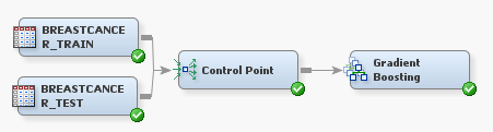
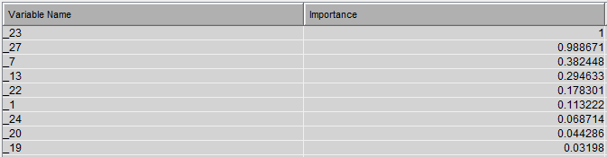
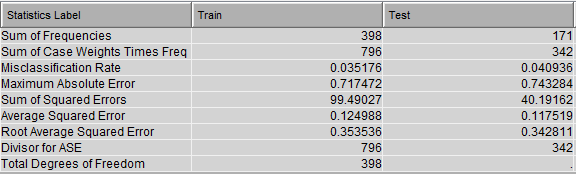
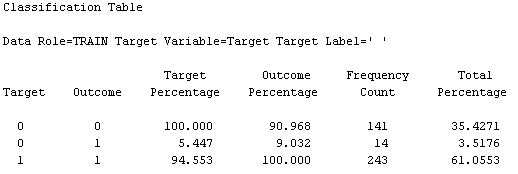
For the Gradient Boosting node, set Seed = 29, set Shrinkage = 0.01, and set Train Proportion = 100.
This diagram results in the following variable importance and misclassification against training & testing data:
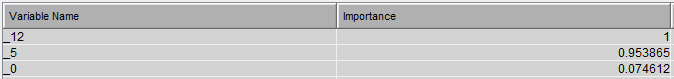
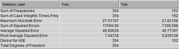
b) Fit a gradient boosting regression model.
Again, there is not a gradient boosting procedure available in Base SAS, currently. Create the following diagram in SAS Enterprise Miner:
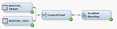
For the Gradient Boosting node, set Seed = 29, set Shrinkage = 0.01, and set Train Proportion = 100.
This diagram results in the following variable importance and root mean squared error against training & testing data:
6.6 Fit an extreme gradient boosting model on taining data and assess against testing data.
a) Fit an extreme gradient boosting classification model.
Fit an extreme gradient boosting classification model on training data and assess the model against the testing data.
For more information on the R code used below, please see the R Tutorial.
proc iml;
  submit / R;
    train = read.csv('C:/Users/breastcancer_train.csv')
    test = read.csv('C:/Users/breastcancer_test.csv')

    library(xgboost)
      set.seed(29)

    xgbMod <- xgboost(data.matrix(subset(train, select = -c(Target))),
                      data.matrix(train$Target), max_depth = 3, nrounds = 2,
                      objective = "binary:logistic", n_estimators = 2500,
                      shrinkage = .01)
    # Prediction on testing data
    predictions <- predict(xgbMod, data.matrix(subset(test, select =
                                                      -c(Target))))
    pred.response <- ifelse(predictions < 0.5, 0, 1)

    # Determine how many were correctly classified
    Results <- ifelse(test$Target == pred.response, "Correct", "Wrong")
    table(Results)
  endsubmit;
quit;
[1] train-error:0.037688
[2] train-error:0.020101
Results
Correct Wrong
165 6Fit an extreme gradient boosting regression model on training data and assess the model against the testing data.
proc iml;
  submit / R;
    train = read.csv('C:/Users/boston_train.csv')
    test = read.csv('C:/Users/boston_test.csv')

    library(xgboost)
      set.seed(29)

    xgbMod <- xgboost(data.matrix(subset(train, select = -c(Target))),
                      data.matrix(train$Target / 50), max_depth = 3,
                      nrounds = 2, n_estimators = 2500, shrinkage = .01)

    # Predict the target in the testing data, remembering to
    # multiply by 50
    prediction = data.frame(matrix(ncol = 0, nrow = nrow(test)))
    prediction$target_hat <- predict(xgbMod,
                                     data.matrix(subset(test,
                                                 select = - c(Target))))*50

    # Compute the squared difference between predicted tip and actual tip
    prediction$sq_diff <- (prediction$target_hat - test$Target)**2

    # Compute the mean of the squared differences (mean squared error)
    # as an assessment of the model
    mean_sq_error <- mean(prediction$sq_diff)
    print(mean_sq_error)
  endsubmit;
quit;
[1] train-rmse:0.146609
[2] train-rmse:0.114851
[1] 36.130796.7 Fit a support vector model on training data and assess against testing data.
a) Fit a support vector classification model.
i) Fit a support vector classification model on training data.
Note: In implementation scaling should be used.
proc import out = train
    datafile = 'C:/Users/breastcancer_train.csv'
    dbms = csv replace;
    getnames = yes;
run;
proc import out = test
    datafile = 'C:/Users/breastcancer_test.csv'
    dbms = csv replace;
    getnames = yes;
run;

/* Fit a support vector classification model */
proc hpsvm data = train noscale;
  input _0-_29 / level = interval;
    target Target / level = nominal;
    code file='hpbreastcancer3.sas';
run;
The HPSVM Procedure
Performance Information
Execution Mode Single-Machine
Number of Threads 4
Data Access Information
Data Engine Role Path
WORK.TRAIN V9 Input On Client
Model Information
Task Type C_CLAS
Optimization Technique Interior Point
Scale NO
Kernel Function Linear
Penalty Method C
Penalty Parameter 1
Maximum Iterations 25
Tolerance 1e-06
Number of Observations Read 398
Number of Observations Used 398
Training Results
Inner Product of Weights 4.68178411
Bias -23.154522
Total Slack (Constraint Violations) 32.0538338
Norm of Longest Vector 4974.69727
Number of Support Vectors 40
Number of Support Vectors on Margin 30
Maximum F 51.3038307
Minimum F -12.975435
Number of Effects 30
Columns in Data Matrix 30
Iteration History
Iteration Complementarity Feasibility
1 1098868.5951 77182929.263
2 1093.5799104 38409.486516
3 399.18453843 11593.175439
4 151.7107168 3299.973204
5 27.079643495 507.367502
6 3.9248813407 34.38606498
7 0.8746382131 3.030830576
8 0.8372881014 3.0263712E-8
9 0.1618601056 5.0387567E-9
10 0.1116181725 2.4391745E-9
11 0.0559596 8.900468E-10
12 0.0340160454 3.048639E-10
13 0.0234420432 1.00729E-10
14 0.015014891 1.898637E-11
15 0.0085767524 9.910531E-11
16 0.003826273 6.162429E-11
17 0.0015691956 5.733211E-11
18 0.0002432757 7.195363E-11
19 1.1925775E-6 1.40731E-10
20 1.9061115E-9 8.307455E-10
Classification Matrix
Training Prediction
Observed 1 0 Total
1 238 5 243
0 8 147 155
Total 246 152 398
Fit Statistics
Statistic Training
Accuracy 0.9673
Error 0.0327
Sensitivity 0.9794
Specificity 0.9484ii) Assess the model against the testing data.
/* Prediction on testing data */
data scored;
    set test;
    %include 'hpbreastcancer3.sas';
run;

/* Determine how many were correctly classified */
data scored;
    set scored;
    if (I_Target = Target) then Result = "Correct";
    else Result = "Wrong";
run;

proc freq data = scored;
  tables Result / nopercent norow nocol;
run;
The FREQ Procedure
Cumulative
Result Frequency Frequency
----------------------------------
Correct 163 163
Wrong 8 171 %include & if-then/else statements | FREQ Procedure
b) Fit a support vector regression model.
Not available in this current release.
6.8 Fit a neural network model on training data and assess against testing data.
a) Fit a neural network classification model.
i) Fit a neural network classification model on training data.
/* Notice we are using new data sets */
  proc import out = train
      datafile = 'C:/Users/digits_train.csv'
      dbms = csv replace;
      getnames = yes;
  run;
  proc import out = test
      datafile = 'C:/Users/digits_test.csv'
      dbms = csv replace;
      getnames = yes;
  run;

/* In order to use the NEURAL Procedure we first need to create a data
   mining database (DMDB) that reflects the original data */
proc dmdb batch data = train
    out = dmtrain
    dmdbcat = digits;
  var _0 - _63;
  class Target;
  target Target;
run;
proc dmdb batch data = test
    out = dmtest
    dmdbcat = digits;
  var _0 - _63;
  class Target;
  target Target;
run;

/* Now we can fit the neural network model */
/* Neural network produces a lot of output which is why here
   "nloptions noprint" is specified */
proc neural data = train dmdbcat = digits random = 29;
  nloptions noprint;
  input _0 - _63 / level = interval;
  target Target / level = nominal;
  archi MLP hidden=100;
  train maxiter = 200;
  score out = out outfit = fit;
  score data = test out = gridout;
run;ii) Assess the model against the testing data.
/* Prediction on testing data */
data scored;
    set gridout;
    rename I_Target = Prediction;
run;

/* This produces a confusion matrix */
proc freq data = scored;
    tables Target*Prediction / nopercent norow nocol;
run;
The FREQ Procedure
Table of Target by Prediction
Target Prediction(Into: Target)
Frequency|0 |1 |2 |3 |4 | Total
---------+--------+--------+--------+--------+--------+
0 | 58 | 0 | 0 | 0 | 0 | 58
---------+--------+--------+--------+--------+--------+
1 | 1 | 56 | 0 | 0 | 0 | 58
---------+--------+--------+--------+--------+--------+
2 | 0 | 0 | 58 | 0 | 0 | 58
---------+--------+--------+--------+--------+--------+
3 | 0 | 0 | 0 | 58 | 0 | 59
---------+--------+--------+--------+--------+--------+
4 | 0 | 0 | 0 | 0 | 51 | 54
---------+--------+--------+--------+--------+--------+
5 | 0 | 0 | 0 | 0 | 0 | 59
---------+--------+--------+--------+--------+--------+
6 | 0 | 0 | 0 | 0 | 0 | 41
---------+--------+--------+--------+--------+--------+
7 | 0 | 0 | 0 | 0 | 0 | 51
---------+--------+--------+--------+--------+--------+
8 | 0 | 4 | 0 | 0 | 0 | 45
---------+--------+--------+--------+--------+--------+
9 | 0 | 0 | 0 | 0 | 0 | 57
---------+--------+--------+--------+--------+--------+
Total 59 60 58 58 51 540
(Continued)
Table of Target by Prediction
Target Prediction(Into: Target)
Frequency|5 |6 |7 |8 |9 | Total
---------+--------+--------+--------+--------+--------+
0 | 0 | 0 | 0 | 0 | 0 | 58
---------+--------+--------+--------+--------+--------+
1 | 0 | 1 | 0 | 0 | 0 | 58
---------+--------+--------+--------+--------+--------+
2 | 0 | 0 | 0 | 0 | 0 | 58
---------+--------+--------+--------+--------+--------+
3 | 1 | 0 | 0 | 0 | 0 | 59
---------+--------+--------+--------+--------+--------+
4 | 1 | 1 | 0 | 1 | 0 | 54
---------+--------+--------+--------+--------+--------+
5 | 58 | 0 | 0 | 0 | 1 | 59
---------+--------+--------+--------+--------+--------+
6 | 0 | 41 | 0 | 0 | 0 | 41
---------+--------+--------+--------+--------+--------+
7 | 1 | 0 | 50 | 0 | 0 | 51
---------+--------+--------+--------+--------+--------+
8 | 0 | 0 | 0 | 39 | 2 | 45
---------+--------+--------+--------+--------+--------+
9 | 2 | 0 | 0 | 2 | 53 | 57
---------+--------+--------+--------+--------+--------+
Total 63 43 50 42 56 540b) Fit a neural network regression model.
i) Fit a neural network regression model on training data.
proc import out = train
    datafile = 'C:/Users/boston_train.csv'
    dbms = csv replace;
    getnames = yes;
run;
proc import out = test
    datafile = 'C:/Users/boston_test.csv'
    dbms = csv replace;
    getnames = yes;
run;

/* In order to use the NEURAL Procedure we first need to create a data
   mining database (DMDB) that reflects the original data */
proc dmdb batch data = train
    out = dmtrain
    dmdbcat = boston;
  var _0 - _12 Target;
  target Target;
run;
proc dmdb batch data = test
    out = dmtest
    dmdbcat = boston;
  var _0 - _12 Target;
  target Target;
run;

/* Now we can fit the neural network model */
/* Neural network produces a lot of output which is why here
   "nloptions noprint" is specified */
proc neural data = train dmdbcat = boston random = 29;
  nloptions noprint;
  archi MLP hidden=100;
  input _0 - _12 / level = interval;
  target Target / level = interval;
  train maxiter = 250;
  score data = test outfit = netfit out = gridout;
run;ii) Assess the model against the testing data.
/* Prediction on testing data */
data scored(keep = sq_error P_Target Target);
    set gridout;
    sq_error = (P_Target - Target)**2;
run;

/* Determine mean squared error */
proc means data = scored mean;
var sq_error;
run;
The MEANS Procedure
Analysis Variable : sq_error
Mean
------------
16.1149499
------------7 Unsupervised Machine Learning
7.1 KMeans Clustering
proc import out = iris
    datafile = 'C:/Users/iris.csv'
    dbms = csv replace;
    getnames = yes;
run;

data iris;
    length Species $ 20;
    set iris;
    if (Target = 0) then Species = "Setosa";
    if (Target = 1) then Species = "Versicolor";
    if (Target = 2) then Species = "Virginica";
run;

proc fastclus data=iris maxclusters=3 out=kmeans random = 29 noprint;
    var PetalLength PetalWidth SepalLength SepalWidth;
run;

proc freq data = kmeans;
    tables Species*Cluster / nopercent nocol norow;
run;
The FREQ Procedure
Table of Species by CLUSTER
Species CLUSTER(Cluster)
Frequency | 1| 2| 3| Total
-----------+--------+--------+--------+
Setosa | 0 | 50 | 0 | 50
-----------+--------+--------+--------+
Versicolor | 0 | 0 | 50 | 50
-----------+--------+--------+--------+
Virginica | 33 | 0 | 17 | 50
-----------+--------+--------+--------+
Total 33 50 67 1507.2 Spectral Clustering
For more information on the R code used below, please see the R Tutorial.
proc iml;
  submit / R;
    iris = read.csv('C:/Users/iris.csv')
      iris$Species = ifelse(iris$Target == 0, "Setosa",
                            ifelse(iris$Target == 1, "Versicolor",
                                   "Virginica"))
      features <- as.matrix(subset(iris, select = c(PetalLength,
                                                    PetalWidth, SepalLength,
                                                    SepalWidth)))
    library(kernlab)
    set.seed(29)
    spectral <- specc(features, centers = 3, iterations = 10,
                      nystrom.red = TRUE)
    labels <- as.data.frame(spectral)
    table(iris$Species, labels$spectral)
  endsubmit;
quit;
              1  2  3
  Setosa     50  0  0
  Versicolor  0 47  3
Virginica 0 3 477.3 Ward Hierarchical Clustering
proc import out = iris
  datafile = 'C:/Users/iris.csv'
  dbms = csv replace;
  getnames = yes;
run;

data iris;
  length Species $ 20;
  set iris;
    if (Target = 0) then Species = "Setosa";
    if (Target = 1) then Species = "Versicolor";
    if (Target = 2) then Species = "Virginica";
run;

proc cluster data = iris method = ward print=15 ccc pseudo noprint;
   var petal: sepal:;
   copy species;
run;

proc tree noprint ncl=3 out=out;
   copy petal: sepal: species;
run;

proc freq data = out;
  tables Species*Cluster / nopercent norow nocol;
run;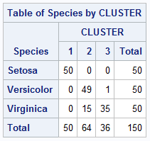
7.4 DBSCAN
For more information on the R code used below, please see the R Tutorial.
proc iml;
  submit / R;
    iris = read.csv('C:/Users/iris.csv')
      iris$Species = ifelse(iris$Target == 0, "Setosa",
                            ifelse(iris$Target == 1, "Versicolor",
                                   "Virginica"))
      features <- as.matrix(subset(iris, select = c(PetalLength,
                                                    PetalWidth, SepalLength,
                                                    SepalWidth)))
    library(dbscan)
      set.seed(29)
    dbscan <- dbscan(features, eps = 0.5)
    labels <- dbscan$cluster
    table(iris$Species, labels)
  endsubmit;
quit;
labels
0 1 2
Setosa 1 49 0
Versicolor 6 0 44
Virginica 10 0 407.5 Self-organizing map
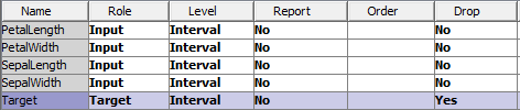
Currently, there is not a self-organizing map procedure available in Base SAS. Therefore, the best method to create a self-organizing map as of now is using SAS Enterprise Miner. First, you need to read in the Iris data set, setting the Species/Target variable to be dropped before investigation.
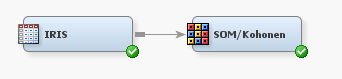
Then create the following diagram in SAS Enterprise Miner:
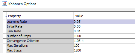
For the SOM/Kohonen node set the following options:
- Choose the Kohonen SOM method.
- Set row and column to both be 4.
- Under the “Kohonen” options section, set “Use Defaults” to “No”, and open the Kohonen Options window by clicking the … box.
- Set the following options in the popup window:
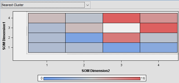
This model produces the following output which is similar to the output of R and Python:
8 Forecasting
8.1 Fit an ARIMA model to a timeseries.
a) Plot the timeseries.
/* Read in new data set */
proc import out = air
  datafile = 'C:/Users/air.csv'
  dbms = csv replace;
  getnames = yes;
run;

proc timeseries data = air plot = series;
    id date interval = month;
    var air;
run;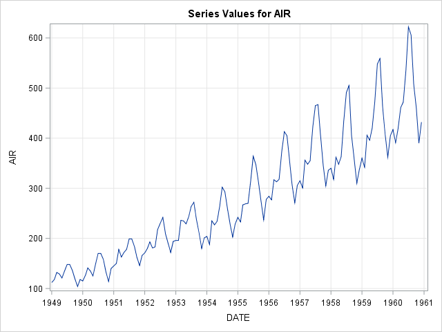
b) Fit an ARIMA model and predict 2 years (24 months).
The output of this code has been limited for space reasons.
proc arima data = air;
    identify var = air(1,12) noprint;
    estimate q=(1)(12) noint method=ml noprint;
    forecast id=date interval=month out=forecast;
run;

/* SAS automatically predicts 2 years out and plots the predictions */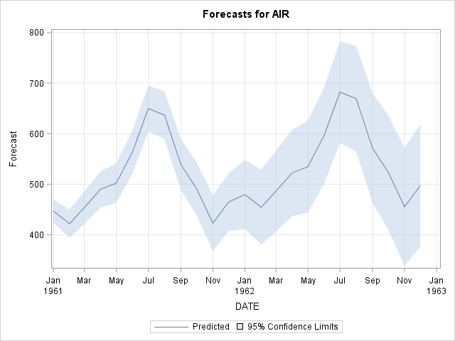
8.2 Fit a Simple Exponential Smoothing model to a timeseries.
a) Plot the timeseries.
proc import out = usecon
  datafile = 'C:/Users/usecon.csv'
  dbms = csv replace;
  getnames = yes;
run;
proc timeseries data = usecon plot = series;
    id date interval = month;
    var petrol;
run;
The TIMESERIES Procedure
Input Data Set
Name WORK.USECON
Label
Time ID Variable DATE
Time Interval MONTH
Length of Seasonal Cycle 12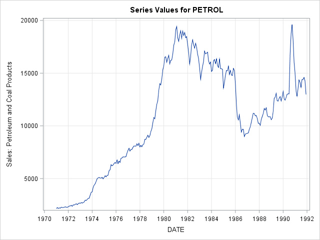
b) Fit a Simple Exponential Smoothing model, predict 2 years (24 months) out and plot predictions.
proc esm data = usecon out = forecast lead = 24 plot = forecasts;
    id date interval = month;
    forecast petrol / model = simple;
run;
The ESM Procedure
Input Data Set
Name WORK.USECON
Label
Time ID Variable DATE
Time Interval MONTH
Length of Seasonal Cycle 12
Forecast Horizon 24
Variable Information
Name PETROL
Label
First JAN1971
Last DEC1991
Number of Observations Read 252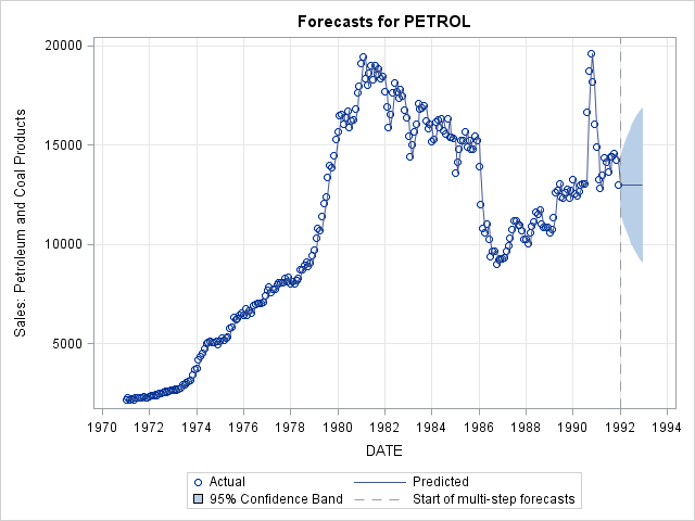
8.3 Fit a Holt-Winters model to a timeseries.
a) Plot the timeseries.
proc timeseries data = usecon plot = series;
    id date interval = month;
    var vehicles;
run;
The TIMESERIES Procedure
Input Data Set
Name WORK.USECON
Label
Time ID Variable DATE
Time Interval MONTH
Length of Seasonal Cycle 12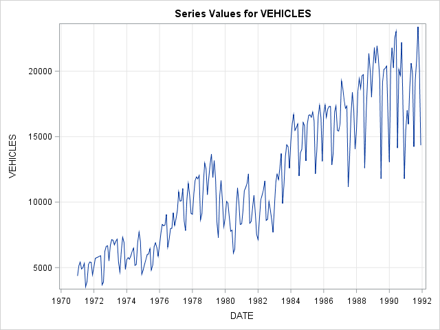
b) Fit a Holt-Winters additive model, predict 2 years (24 months) out and plot predictions.
proc esm data = usecon out = forecast lead = 24 plot = forecasts;
    id date interval = month;
    forecast vehicles / model = addwinters;
run;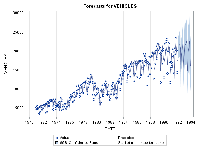
9 Model Evaluation & Selection
9.1 Evaluate the accuracy of regression models.
a) Evaluation on training data.
proc import out = train
    datafile = 'C:/Users/boston_train.csv'
    dbms = csv replace;
    getnames = yes;
run;
proc import out = test
    datafile = 'C:/Users/boston_test.csv'
    dbms = csv replace;
    getnames = yes;
run;

/* Random Forest Regression Model */
ods select none;
proc hpforest data = train ;
    input _0-_12 / level = interval;
    target Target / level = interval;
    save file = 'rfMod.bin';
run;
ods select all;

/* Evaluation on training data  */
ods select none;
proc hp4score data = train;
    score file = 'rfMod.bin' out = scored_train;
run;
ods select all;

/* Determine coefficient of determination score */
proc iml;
  use scored_train;
    read all var _ALL_ into data;
  close scored_train;
  tip = data[,1];
  pred_rf = data[,2];
  r2_rf = 1 - ( (sum((tip - pred_rf)##2)) / (sum((tip - mean(tip))##2)) );
  print(r2_rf);
quit;
r2_rf
0.9751727b) Evaluation on testing data.
/* Random Forest Regression Model (rfMod) */

/* Evaluation on testing data  */
ods select none;
proc hp4score data = test;
    score file = 'rfMod.bin' out = scored_test;
run;
ods select all;

/* Determine coefficient of determination score */
proc iml;
  use scored_test;
    read all var _ALL_ into data;
  close scored_test;
  tip = data[,1];
  pred_rf = data[,2];
  r2_rf = 1 - ( (sum((tip - pred_rf)##2)) / (sum((tip - mean(tip))##2)) );
  print(r2_rf);
quit;
r2_rf
0.8892346The formula used here for the coefficient score is based off the Python skearn formula for r2_score.
9.2 Evaluate the accuracy of classification models.
a) Evaluation on training data.
proc import out = train
    datafile = 'C:/Users/digits_train.csv'
    dbms = csv replace;
    getnames = yes;
run;
proc import out = test
    datafile = 'C:/Users/digits_test.csv'
    dbms = csv replace;
    getnames = yes;
run;

/* Random Forest Classification Model */
ods select none;
proc hpforest data = train;
    input _0-_63 / level = interval;
    target Target / level = nominal;
    save file = 'rfMod.bin';
run;

/* Evaluation on training data */
proc hp4score data = train;
    score file = 'rfMod.bin' out = scored;
run;
ods select all;

data scored(keep = Target I_Target correct);
    set scored;
    correct = (I_Target = Target);
run;

/* Determine accuracy score */
proc iml;
    use scored;
      read all var _ALL_ into data;
    close scored;

    accuracy_forest = (1/nrow(data)) * sum(data[,2]);

    print(accuracy_forest);
quit;
accuracy_forest
1b) Evaluation on testing data.
/* Random Forest Classification Model (rfMod) */

/* Evaluation on testing data */
ods select none;
proc hp4score data = test;
    score file = 'rfMod.bin' out = scored;
run;
ods select all;

data scored(keep = Target I_Target correct);
    set scored;
    correct = (I_Target = Target);
run;

/* Determine accuracy score */
proc iml;
    use scored;
      read all var _ALL_ into data;
    close scored;

    accuracy_forest = (1/nrow(data)) * sum(data[,2]);

    print(accuracy_forest);
quit;
accuracy_forest
0.9722222The formula used here for the accuracy score is based off the Python skearn formula for accuracy_score.
Appendix
1 Built-in SAS Data Types
2 SAS Procedures
Alphabetical Index
Data Frame
A two-dimensional tabular structure with labeled axes (rows and columns), where data observations are represented by rows and data variables are represented by columns.
Dictionary
An associative array which is indexed by keys which map to values. Therefore, a dictionary is an unordered set of key:value pairs where each key is unique. In SAS, a dictionary can be implemented using a hash table. Please see the following example.
/* Results will be displayed in the log */
data class_dict;
declare hash mydict();
mydict.defineKey("Name");
mydict.defineData("Age");
mydict.defineDone();
do while (not eof);
  set sashelp.class end = eof;
  rc = mydict.add();
  output;
end;
Name = 'James';
rc = mydict.find();
put rc= Name= Age=;